CS6140 Machine Learning
HW3 Generative Models
EM class notes, Other EM
notes1, notes4,
notes5
Multivariate
Normal, Multivariate
- mariginal and conditional, Correlation
Coefficient
You have to
write your own code, but it is ok to discuss or look up specific
algorithmic/language code details. Before starting coding, make
sure to understand :
- how
2-dim Gaussians work
- Naive
Bayes independence of features, thus the product of
probabilities
- languages
like Python or Matlab or R can help immensely in dealing with
multidimensional data, including the means and covariances in
2-dim.
- E and M
steps for EM algorithm. You can look into existing
EM code for help.
PROBLEM 1 GDA [50 points]
Run the Gaussian Discriminant Analysis on the spambase data. Use the
k-folds from the previous problem (1 for testing, k-1 for training,
for each fold)
Since you have 57 real value features, each of the 2gaussians
(for + class and for - class) will have a mean vector with 57
components, and a they will have
- either a common (shared) covariance matrix size 57x57. This
covariance is estimated from all training data (both classes)
- or two separate covariance 57x57 matrices (estimated
separately for each class)
(you can use a Matlab or Python of Java built in function to
estimated covariance matrices, but the estimator is easy to code
up).
Looking at the training and testing performance, does it appear that
the gaussian assumption (normal distributed data) holds for this
particular dataset?
PROBLEM 2: Naive Bayes [50 points]
Create a set of Naive Bayes classifiers for detecting e-mail spam and test the classifiers on the Spambase dataset via 10-fold cross validation.
2.1: Build the classifier(s)
Create three distinct Naive Bayes classifiers by varying the likelihood distribution. In particular, try:
Modeling the likelihood using a Bernoulli distribution
Modeling the likelihood using a Gaussian distribution
Modeling the likelihood non-parameterically / histogram (optional)
For real-valued features, a Bernoulli likelihood may be obtained by thresholding against a scalar-valued statistic, such as the sample mean \(\mu\). Similarly, a Gaussian likelihood function can be obtained by estimating the [class conditional] expected value \(\mu\) and variance \(\sigma\). For the non-parameteric setting, model the feature distribution either with a kernel density estimate (KDE) or a histogram.
Bernoulli example: Consider some threshold \(\mu \in \mathbb{R}\). To compute the conditional probability of a feature \(f_i\), compute the fraction by which \(f_i\) is above or below \(\mu\) over all the data within its class. In other words, for feature \(f_i\) with expected value \(\mu_i\), estimate: \[ P(f_i \leq \mu_i \mid \text{spam} ) \text{ and } P(f_i > \mu_i \mid \text{spam} )\] \[ P(f_i \leq \mu_i \mid \text{non-spam} ) \text{ and } P(f_i > \mu_i \mid \text{non-spam} )\] and use these estimated values in your Naive Bayes predictor.
For all the models mentioned, you may want to consider using some kind of additive smoothing technique as a regularizer.
2.2: Evaluate your results
Evaluate the performance of the classifiers using the following three performance summaries.
Error tables: Create a table with one row per fold showing the false positive, false negative, and overall error rates of the classifiers. Add one final row per table yielding the average error rates across all folds.
ROC Curves: Graph the Receiver Operating Characteristic (ROC) curve for each of your classifiers on Fold 1 and calculate their area-under-the-curve (AUC) statistics. You should draw all three curves on the same plot so that you can compare them.
For this problem, the false positive rate is the fraction of non-spam testing examples that are misclassified as spam, while the false negative rate is the fraction of spam testing examples that are misclassified as non-spam.
Context: In many situations, false positive (Type I) and false negative (Type II) errors incur different costs. In spam filtering, for example, a false positive is a legitimate e-mail that is misclassified as spam (and perhaps automatically redirected to a “spam folder” or, worse, auto-deleted) while a false negative is a spam message that is misclassified as legitimate (and sent to one’s inbox).
When using Naive Bayes, one can easily make such trade-offs. For example, in the usual Bayes formulation, with \(\mathbf{x}\) the data vector and \(y\) the class variable, one would predict “spam” if:
\[ P(y = \text{spam} | \mathbf{x}) > P(y = \text{non-spam} | \mathbf{x}) \]
or equivalently, in a log-odds formulation,
\[ \ln(P(y = \text{spam} | \mathbf{x}) / P(y = \text{non-spam} | \mathbf{x})) > 0 \]
However, note that one could choose to classify an e-mail as spam for any threshold \(\tau\), i.e.:
\[ \ln(P(y = \text{spam} | \mathbf{x}) / P(y = \text{non-spam} | \mathbf{x})) > \tau \]
Larger values of \(\tau\) reduce the number of spam classifications, reducing false positives at the expense of more false negatives. Negative values of \(\tau\) have the converse effect.
Most users are willing to accept some false negative examples so long as very few legitimate e-mails are misclassified. Given your classifiers and their ROC curves, what value of \(\tau\) would you choose to deploy in a real email spam filter?
PROBLEM 3 EM Algorithm Description [20 points]
Use this pdf of the EM code demoed
in class. (Alternatively, you can print the code
yourself from an editor).
Annotate on the right the sections of the code with your
explanation of what the code does. Submit as pdf.
PROBLEM 4 : EM on simple data [50 points]
A) The gaussian 2-dim data on file 2gaussian.txt
has
been generated using a mixture of two Gaussians,
each 2-dim, with the parameters below. Run the EM algorithm
with random initial values to recover the parameters.
mean_1 [3,3]); cov_1 =
[[1,0],[0,3]]; n1=2000 points
mean_2 =[7,4]; cov_2 =
[[1,0.5],[0.5,1]]; ; n2=4000 points
You should obtain a result visually like
this (you dont necessarily have to plot it)
B) Same problem for 2-dim data on file 3gaussian.txt , generated using a mixture
of three Gaussians. Verify your findings against the true
parameters used generate the data below.
mean_1 = [3,3] ; cov_1 =
[[1,0],[0,3]]; n1=2000
mean_2 = [7,4] ; cov_2 =
[[1,0.5],[0.5,1]] ; n2=3000
mean_3 = [5,7] ; cov_3 =
[[1,0.2],[0.2,1]] ); n3=5000
PROBLEM 5 [GR only]
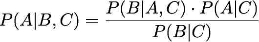
a) Prove that
b) You are given a coin which you know is either fair or
double-headed. You believe
that the a priori odds of it being fair are F to 1; i.e., you
believe that the a priori probability of the coin
being fair is F/(F+1) . You now begin to flip the coin in order to
learn more. Obviously, if you ever see a tail,
you know immediately that the coin is fair. As a function of F, how
many heads in a row would you need to see before becoming convinced
that there is a better than even chance that the coin is
double-headed?
PROBLEM 6 - 30 points
Cheng's
note summarizing E an M steps for this problem.
A.Generate
mixture data (coin flips). Pick a p,r,pi as in the EM
example discussed in class (or in notes). Say p=.75, r=.4, pi=.8,
but you should try this for several sets of values. Generate the
outcome of the coin experiment by first picking a coin (pi
probability for first coin, 1-pi probability for the second coin),
then flip that coin K times (use K=10) with probability of head (p
if first coin is picked, r if the second coin is picked) and
finally write down a 1 if the head is seen, 0 for the tail. Repeat
this M=1000 times or more; so your outcome is a stream of M
sequences of K flips : (1001110001; 0001110001; 1010100101 etc)
B.Infer parameters from data. Now using
the stream of 1 and 0 observed, recover p,r,pi using the EM
algorithm; K is known in advance. Report in a table the parameter
values found by comparison with the ones used to generate data; try
several sets of (p,r,pi). Here are some useful notes,
and other readings (1
, 2
, 3
, 4)
for the coin mixture.
C(more coins, optional). Repeat A) and B)
with T coins instead of two. You will need more mixture parameters.
PROBLEM 7 Naive Bayes with Gaussian Mixtures[Extra Credit]
Rerun the Naive Bayes classifier on Spam Data. For each feature
(1-dim) use a mixture of K Gaussians as your model ; run the EM to
estimate the 3*K parameters for each feature : mean1, var1, w1; mean2,var2,
w2;... meanK,varK,wK; constrained by w1+w2 +...+wK=1.
(You would need a separate mixture for positive and negative data,
for each feature). We observed best results for K=9.
Testing: for each testing point , apply the Naive
Bayes classifier as before: take the log-odd of product of
probabilities over features mixtures (and the prior), separately for
positive side and negative side; use the overall probability ratio
as an output score, and compute the AUC for testing set. Do
this for a 10-fold cross validation setup. Is the overall 10-fold
average AUC better than before, when each feature model was a single
Gaussian?
PROBLEM 8 [Extra Credit]
a) Somebody tosses a fair coin and if the result is heads, you
get nothing, otherwise you get $5. How much would you be pay to
play this game? What if the win is $500 instead of $5?
b) Suppose you play instead the following game: At the beginning
of each game you pay an entry fee of $100. A coin is tossed until
a head appears, counting n = the number of tosses it took to see
the first head. Your reward is 2n (that is: if a head
appears first at the 4th toss, you get $16). Would you be willing
to play this game (why)?
c) Lets assume you answered "yes" at part b (if you did not, you
need to fix your math on expected values). What is the probability
that you make a profit in one game? How about in two games?
d) [difficult] After
about how many games (estimate) the probability of making a profit
overall is bigger than 50% ?
PROBLEM 9 [Extra Credit]
DHS CH2, Pb 43
PROBLEM 10 part 2 [Extra Credit]
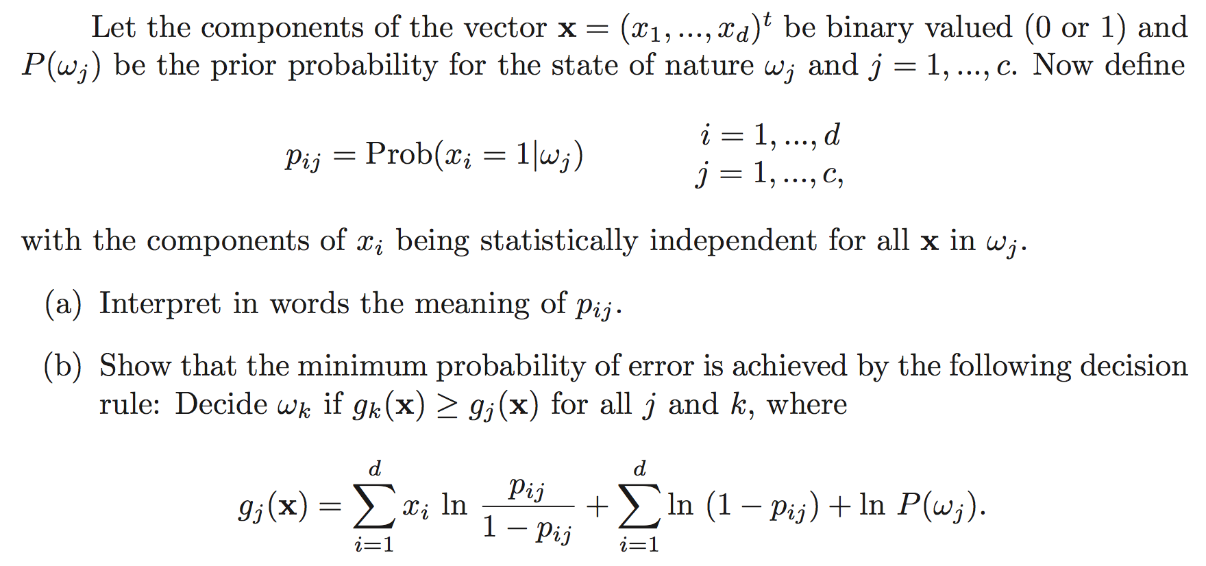
a) DHS CH2, Pb 45
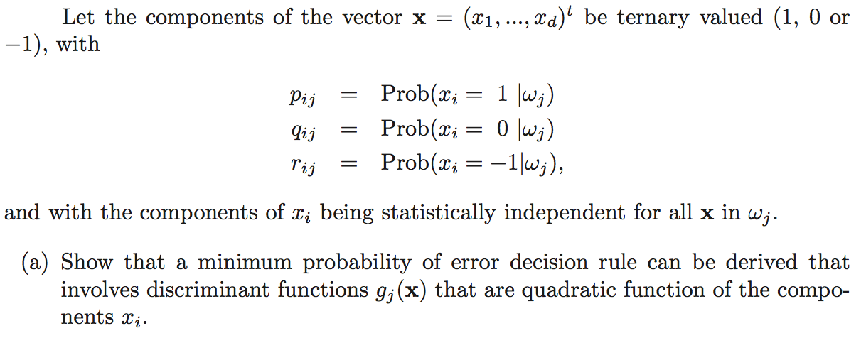
PROBLEM 11 [Extra Credit]
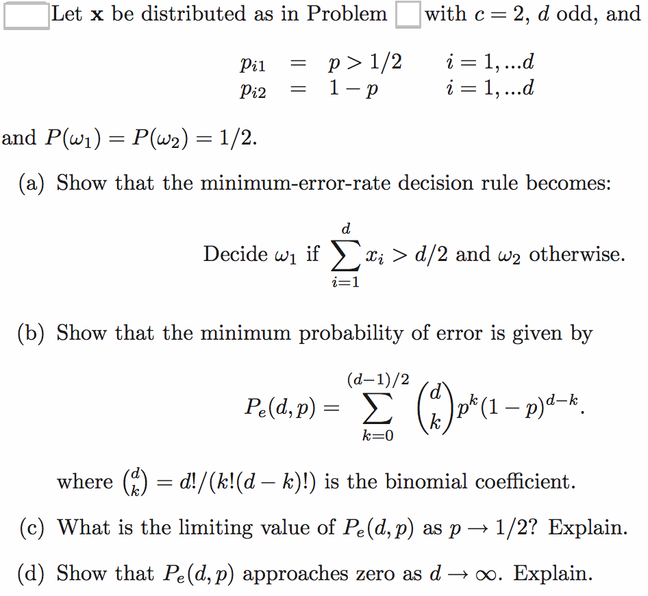
b) DHS CH2, Pb 44
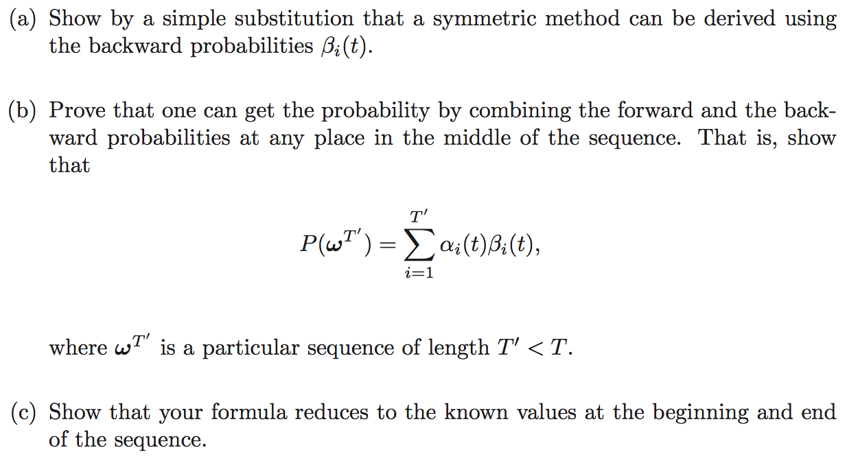
PROBLEM 12 [EXTRA CREDIT, requires independent study of Hidden
Markov Models, DHS ch 3.10]
DHS Pb 3.50 (page 154-155)
The standard method for calculating the probability of a sequence in
a given HMM is to use the forward probabilities αi(t).