CS6140 Machine Learning — Fall 2026

HW3 — Kernels, SVM, Kernel Ridge, PCA, KPCA

Make sure you check the syllabus for the due date. Please use the notations adopted in class.

Instructions. Submit code (Jupyter notebook encouraged) plus a short report with tables and plots. Libraries (numpy, sklearn, matplotlib) are allowed for data handling, plotting, and basic math; the core of any "from scratch" problem must be your own.

Requirements.

• Fill in every TODO_STUDENT blank according to the algorithm steps covered in lecture and the linked materials, and make sure the notebook runs top to bottom without errors.
• Understand the whole notebook — including the provided/given code, not just the blanks you filled in — well enough to explain any part of it during office hours.

Model/hyperparameter selection. Wherever a problem asks you to choose among kernels, hyperparameters, or a dimension (Problem 1's kernel grid, Problem 3's kernel + regularization, Problem 5's T), split off a validation set and pick using validation performance only. Report the test-set number once, for the configuration you already chose — never pick a configuration by looking at test performance.

Datasets. Links are relative to ../../data/.... Used here: Spambase, polluted Spambase, the Digits dataset (images / HAAR features), the WAVE set (waveX, waveY) and CRESCENT set (crescentX, crescentY), and the 2-D TwoSpirals (used in Problems 2 and 5, binary, label ∈ {−1,+1}) / ThreeCircles (Problem 5 only — despite the shared 2-D-points file format, this is a balanced 3-class dataset, label ∈ {−1,0,+1}, chance ≈ 33%, not 50%) sets.

Starter code. For each problem where a library counterpart exists, the starter notebook gives you the full data/eval pipeline and asks you to fill in two things: a short library-call baseline (a quick sanity-check number, using a well-known library function) and the from-scratch algorithm steps, evaluated the same way — your from-scratch number should land on or near the library one. The one exception is Problem 1, which is the library problem — it has no from-scratch counterpart to compare against (that's Problem 2). Answers to the (THEORY) problems may be written directly in the notebook (e.g. a markdown cell) rather than a separate document, as long as they include any equation, plot, or illustration the answer depends on — not prose alone.

PROBLEM 1 — SVM (library)   [30 points]

Use an SVM library of your choice (e.g. LIBSVM, scikit-learn). Try several kernels, including polynomial and RBF; report results.

• Part A (binary): Spambase.
• Part B (multiclass, required): the Digits dataset. If your SVM package is binary only, write a multiclass wrapper — one-vs-the-rest (10 classifiers) or all-pairs voting (45 classifiers, predict by most wins).

Library calls: sklearn.svm.SVC, sklearn.multiclass.OneVsRestClassifier (this problem is library-only by design — there's no from-scratch counterpart required here; see PROBLEM 2 for the from-scratch SVM).

PROBLEM 2 — SVM from scratch (Simplified SMO)   [70 points]

Implement your own SVM solver using the Simplified SMO algorithm: see the CS229 Simplified SMO notes — iterate over all α_i, and whenever α_i violates the KKT conditions pick a random α_j among the rest and jointly optimize the pair. (The full Platt SMO algorithm — writeup here — adds an error cache and pair-selection heuristics for speed; that fuller version is optional below, not required.) Write your solver so it only ever looks at a precomputed kernel (Gram) matrix, never raw features directly — that way the same code works for any kernel.

• Part A (linear kernel, correctness check): run on the TwoSpirals data (same file as Problem 5). Recover the primal weight vector w = ∑α_iy_ix_i and compare it directly against a library linear SVM's weight vector (e.g. SVC(kernel='linear').coef_) — this validates your optimizer even though a linear kernel classifies this data poorly (TwoSpirals is not linearly separable by construction).
• Part B (RBF kernel, required): rerun the identical solver with an RBF Gram matrix in place of the linear one, on the same TwoSpirals train/test split. Compare accuracy against a library RBF-SVM on the same split — both should solve it almost perfectly, which is the actual point of the kernel trick (and of picking this dataset instead of Spambase, where a linear kernel already does about as well as RBF and so wouldn't show much).

Note: the "stop once a fixed number of sweeps pass with no change" stopping rule in the Simplified SMO notes is not guaranteed to trigger on noisy, non-separable data. Cap the total number of sweeps (e.g. 300) so your run time stays bounded regardless of whether that rule ever fires — without a cap this can run for a very long time.

[optional] Run the same solver on Spambase or ThreeCircles; implement the full Platt SMO heuristics (error cache, entire-set/non-bound alternation, second-choice pair selection) instead of the simplified version; run it on Digits via a multiclass wrapper.

Library calls: sklearn.svm.SVC (linear and RBF kernels), matching Problem 1's library baseline.

PROBLEM 3 — Kernel Ridge Regression from scratch   [50 points]

Implement a kernel ridge regression wrapper with fit(X, y) and predict(X); the initializer selects the kernel (linear, polynomial, RBF) and its hyperparameters (regularization λ solved as α = (K + λI)^-1y). The kernel evaluation may use a library, but the rest must be from scratch. Check your implementation against a library baseline (e.g. sklearn.kernel_ridge.KernelRidge) at the same kernel/hyperparameters.

• Fit the WAVE data with linear, RBF, and polynomial kernels; tune hyperparameters on a validation split.
• Evaluate train/test MSE for each kernel and plot predicted vs true coordinates.
• Repeat for the CRESCENT data. Explain which kernel did better on each and why.

Library calls: sklearn.kernel_ridge.KernelRidge.

PROBLEM 4 — PCA from scratch (feature corruption & rescue)   [40 points]

Using the polluted Spambase dataset (original points, many extra junk / duplicated features):

• A) Train a classifier on the raw polluted features and observe the drop in performance relative to the same classifier on the original, unpolluted 57-feature Spambase — fit and report that unpolluted control inside this notebook, not just from memory of HW2's numbers. Use logistic regression (from HW2) as the downstream classifier.
• B) Run PCA (a library is allowed here) to reduce to ~100 features, then retrain. Apply PCA consistently to train and test (fit on train, apply the stored transform to test). Explain the improvement.
• C) Implement your own PCA and rerun the classifier on your PCA features.

Library calls: sklearn.decomposition.PCA, sklearn.linear_model.LogisticRegression.

PROBLEM 5 — Kernel PCA + linear classifier   [60 points]

Datasets: 1000 2-D points each — TwoSpirals (binary, chance ≈ 50%) and ThreeCircles (a balanced 3-class dataset despite the shared file format, chance ≈ 33%). Report chance level alongside accuracy so the two datasets' numbers aren't compared as if both were binary.

• A) Train a linear/logistic classifier and confirm it fails (high error, near chance) on the raw 2-D data.
• B) Run Kernel PCA with a Gaussian kernel (e.g. γ=1) to obtain a T-dimensional representation (build the kernel matrix, center it, eigendecompose, project — including the out-of-sample centering formula for new/test points). Check your implementation against a library baseline (e.g. sklearn.decomposition.KernelPCA) at your chosen T.
• C) Retrain the linear classifier on the kernelized features, sweeping T over a few values (e.g. 2, 5, 10, 20, 50). Choose T on a validation split — e.g. the smallest T reaching some accuracy bar you define as "good" (such as 90% validation accuracy) — and confirm that choice once on the held-out test set. The two datasets are not equally hard, so don't expect the same T for both.

Library calls: sklearn.decomposition.KernelPCA, sklearn.linear_model.LogisticRegression.

PROBLEM 6 (THEORY) — Choosing the RBF Bandwidth in Kernel Ridge Regression   [25 points]

Fit your PROBLEM 3 kernel ridge regression on WAVE or CRESCENT with an RBF kernel at a very small bandwidth vs. a much larger bandwidth. With a very small bandwidth, the fitted curve passes almost exactly through every training point, with wild oscillations between them; with a larger bandwidth, it looks like a smooth curve that doesn't hit every point exactly, but tracks the overall trend.

In a short written answer, explain this pattern, and propose how to choose the bandwidth properly (i.e., not by eye and not by minimizing training error).

PROBLEM 7 (THEORY) — One-vs-Rest SVM Ambiguity in Multiclass Regions   [25 points]

Your PROBLEM 1 one-vs-rest multiclass SVM wrapper trains one binary SVM per class and predicts using whichever classifier gives the most confident "positive" score. For most test points this works fine, but for points near the boundary between three or more classes, it is possible for all the binary classifiers to output a negative ("not this class") decision, leaving no clear winner — or, conversely, for multiple classifiers to claim the point positively.

In a short written answer, explain why one-vs-rest can produce this kind of ambiguous region, and propose whether switching to a one-vs-one (all-pairs) voting scheme would fix it.

PROBLEM 8 — SVM-SMO on the Digits Dataset   [optional, no credit]

Instead of a library SVM, run your own Problem 2 SMO solver on the Digits dataset. Digits has 10 classes and your SMO is a binary classifier, so you need a multiclass wrapper on top of it — choose one of:

• One-vs-the-rest: train 10 binary SMO classifiers, one per class.
• ECOC on top of SMO: same idea as ECOC boosting, just with your SMO solver as the base binary classifier.
• All-pairs voting: train all (10 choose 2) = 45 one-vs-one models (e.g. the "7 vs 9" model trains/tests only on points labeled 7 or 9). At test time, run all 45 models and predict the class with the most wins; break ties using the direct head-to-head match.

Digits is learnable enough that you can subsample the training set (e.g. 10–20% per class) to keep runtime down — but evaluate on the full test set.

PROBLEM 9 — The Full Platt SMO Algorithm   [optional, no credit]

Problem 2 uses the CS229 Simplified SMO algorithm (random second-variable selection, no error cache). Extra credit for implementing the full Platt SMO heuristics instead, following the Platt SMO paper:

• a maintained error cache, so you're not recomputing E_i from scratch for every point on every sweep;
• the entire-set / non-bound-subset alternation (sweep all points, then only the non-bound ones, alternating until neither changes anything);
• the second-choice heuristic for picking α_j — maximize |E_i − E_j| among non-bound points first, falling back to a scan over the non-bound set and then the full set if that makes no progress (instead of Problem 2's uniform-random pick).

Reference implementations already exist in this course's materials (6_SVM_kernels/code_HW6/bingyu/SVM/SVM.py, SMO.java) if you want to check your work against them — but implement your own rather than copying them.

PROBLEM 10 — Solve the Dual with a Library QP Solver   [optional, no credit]

Same problem as Problem 2, but instead of SMO, solve the SVM dual directly with a general-purpose quadratic-programming solver (e.g. cvxopt.solvers.qp in Python, or an equivalent in Matlab/Java/C). Compare the resulting α's and accuracy against your SMO solution.

PROBLEM 11 — Six-Point Hyperplane by Inspection   [optional, no credit]

Consider the following 6 points in 2-D, for two classes:

class 0:   (1,1)   (2,2)   (2,0)
class 1:   (0,0)   (1,0)   (0,1)

a) Plot these 6 points, construct the optimal hyperplane by inspection and intuition (give W, b) and calculate the margin.
b) Which points are support vectors?
c) [Extra credit] Construct the hyperplane by solving the dual optimization problem using the Lagrangian. Compare with part (a).

PROBLEM 12 — The Dual Constraint 0 ≤ α ≤ C/m   [optional, no credit]

Explain why 0 ≤ α ≤ C/m is a constraint in the dual optimization with slack variables (hint: read the Burges SVM tutorial first). Distinguish three cases, and explain each in terms of the classification and the constraints: a) α = 0; b) 0 < α < C/m; c) α = C/m. This has been discussed in class and in the SVM notes; a detailed, rigorous explanation is expected, not just a restatement of the three cases.

PROBLEM 13 — VC Dimension   [optional, no credit]

What is the VC dimension of an SVM with a linear kernel?

PROBLEM 14 — LDA Instead of PCA   [optional, no credit]

Problem 4 rescues polluted Spambase with PCA. Run LDA instead of PCA before the downstream logistic regression classifier — you can use a library LDA implementation (e.g. sklearn.discriminant_analysis.LinearDiscriminantAnalysis). Compare accuracy against Problem 4's PCA result.

PROBLEM 15 — DHS Chapter 5   [optional, no credit]

Pick a problem from DHS (Duda, Hart & Stork, Pattern Classification) chapter 5 (linear discriminant functions / SVMs) that isn't already covered above, and solve it. If you're not sure which one to pick, ask.

PROBLEM 16 — t-SNE Dimensionality Reduction   [optional, no credit]

t-SNE isn't a kernel method, but it rhymes with this HW's PCA/KPCA problems: another way to turn high-dimensional data into something a 2-D plot (or a simple downstream classifier) can actually work with — and unlike PCA, it's built specifically to preserve local neighborhood structure, at the cost of not being a linear projection at all.

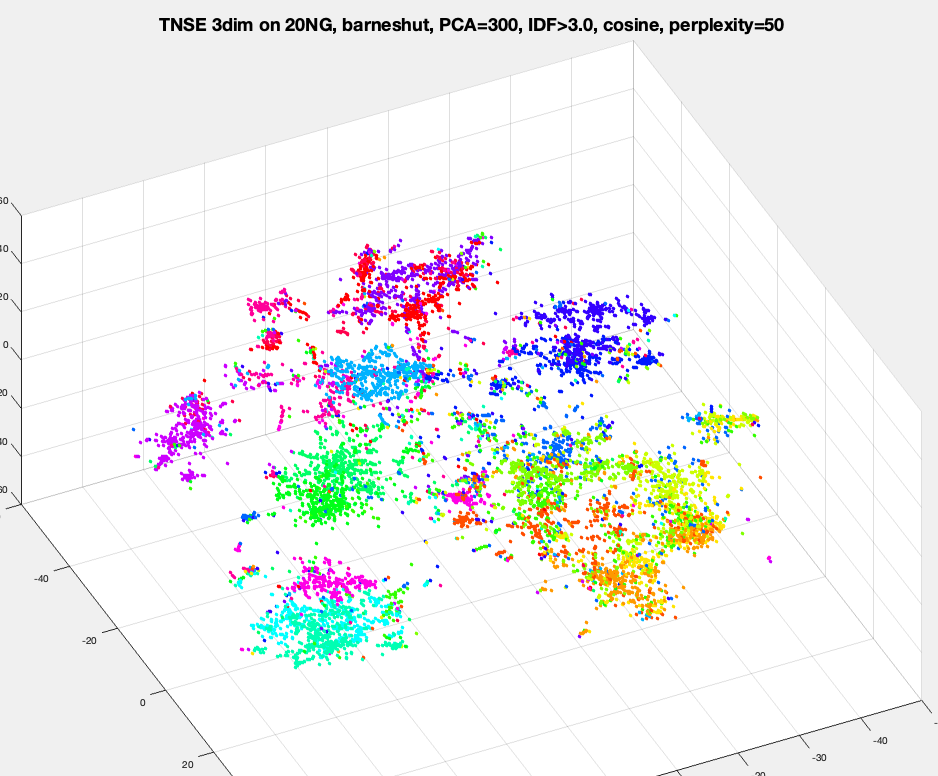
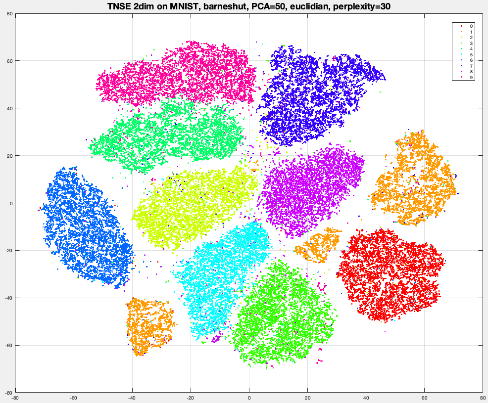
Part A (library). Run a library t-SNE (e.g. sklearn.manifold.TSNE) on MNIST and/or 20 Newsgroups, project to 2 or 3 dimensions, and scatter-plot the points colored by label. Try a few perplexity values (e.g. 5, 20, 100) and see how the picture changes. Here's what a good result looks like — each color is a different digit/newsgroup, and they should separate into fairly clean clusters:

Part B (from scratch, harder). Implement t-SNE yourself. We're deliberately not giving you code here — go read Laurens van der Maaten's own t-SNE page (the original author; it has the paper, reference implementations in several languages, and FAQ) and work from that. At a high level, the algorithm is:

1. Reduce the input to ~50 dimensions with PCA first (t-SNE itself is for refining local structure, not for crunching raw high-dimensional data efficiently).
2. Compute the pairwise squared-distance matrix in that reduced input space.
3. For each point i, binary-search a per-point bandwidth so the resulting conditional distribution over its neighbors has a fixed "effective number of neighbors" — matching a target perplexity via that distribution's entropy.
4. Symmetrize and normalize into one joint distribution P over all pairs, in the original high-dimensional space.
5. Initialize a random low-dimensional embedding Y; define Q as the (normalized) Student-t similarities between points in that embedding — the heavy tail is what gives t-SNE room to spread out clusters that would otherwise collapse on top of each other.
6. Gradient-descend (momentum/adaptive gains help a lot in practice) on KL(P ‖ Q), nudging points in Y until the low-dimensional similarities match the high-dimensional ones as well as they can.
7. Every few iterations, re-center Y and check in (plot it, watch the KL-divergence trend down) — this is as much art as it is algorithm.

Run your implementation on MNIST (or a manageable subsample of it) and compare your scatter plot against Part A's library result.

Library calls: sklearn.manifold.TSNE (Part A only — Part B is the from-scratch counterpart).