Make sure you check the syllabus for the due date. Please use the notations adopted in class.
Instructions. Submit code (Jupyter notebook encouraged) plus a short report with tables and plots. Libraries (numpy, scipy, sklearn, matplotlib) are allowed for data handling, plotting, and math functions such as Gaussian/Binomial densities and random number generation; the core estimation / EM logic of each "from scratch" problem must be your own.
Requirements.
Datasets. Paths are relative to the course data folder (../../data/...). Core dataset: Spambase (spambase/spambase.data, binary classification, one file — split yourself for k-fold / 10-fold CV). Problem 3 uses the generated files 2gaussian.txt and 3gaussian.txt in this folder. Problem 4 uses data you generate yourself — no file is provided. Problem 5 reuses HW1's Housing set (housing_train.txt / housing_test.txt, pre-split regression data). The optional Kernel Fisher Discriminant problem reuses HW3's TwoSpirals/ThreeCircles (TwoSpirals/twoSpirals.txt, TwoSpirals/threecircles.txt).
Starter code. For each problem where a library counterpart exists, the starter notebook gives you the full data/eval pipeline and asks you to fill in two things: a short library-call baseline (a quick sanity-check number, using a well-known library function) and the from-scratch algorithm steps, evaluated the same way — your from-scratch number should land on or near the library one. Not every problem has a library counterpart to compare against (PROBLEM 4, and the non-parametric variant within PROBLEM 2, are the exceptions below); those are marked accordingly. Answers to the (THEORY) problems may be written directly in the notebook (e.g. a markdown cell) rather than a separate document, as long as they include any equation, plot, or illustration the answer depends on — not prose alone.
Perform Gaussian Discriminant Analysis on the Spambase data with k-fold cross validation. For each fold, use 1 fold for testing and k−1 folds for training.
During the analysis, test both of the following covariance assumptions:
Based on the training and testing performance, does it appear that the data are normally distributed?
Library calls: sklearn.discriminant_analysis.LinearDiscriminantAnalysis, sklearn.discriminant_analysis.QuadraticDiscriminantAnalysis.
Create a set of Naive Bayes classifiers for detecting e-mail spam and test them on the Spambase dataset via 10-fold cross validation.
2.1 — Build the classifiers. Create three distinct Naive Bayes classifiers by varying the per-feature likelihood model:
Bernoulli example. Consider a threshold μi ∈ ℝ for feature fi (its class-conditional sample mean). Estimate, over the training data within each class:
P(fi ≤ μi | spam) and
P(fi > μi | spam)
P(fi ≤ μi | non-spam) and
P(fi > μi | non-spam)
and use these estimated probabilities in your Naive Bayes predictor.
Regularize each model so no feature/class combination ever gets a zero probability: for the Bernoulli and Histogram variants (both discrete counts/probability masses), use additive (Laplace) smoothing; for the Gaussian variant, additive smoothing doesn't apply to a continuous density the same way — use a small variance floor instead (add a small ε to every estimated variance so it's never exactly zero).
2.2 — Evaluate and choose a threshold. In spam filtering, false positive (Type I) and false negative (Type II) errors have very different costs: a false positive is a legitimate e-mail misclassified as spam (redirected to a spam folder, or worse, auto-deleted), while a false negative is a spam message that lands in the inbox.
With x the feature vector and y the class label, the usual Bayes decision rule predicts "spam" when P(y=spam|x) > P(y=non-spam|x), i.e., in log-odds form, when
ln( P(y=spam|x) / P(y=non-spam|x) ) > 0
But you may classify as spam under any threshold τ:
ln( P(y=spam|x) / P(y=non-spam|x) ) > τ
Larger τ reduces spam classifications (fewer false positives, more false negatives); negative τ has the opposite effect. Most users tolerate some false negatives as long as very few legitimate e-mails are flagged. Using your three classifiers' ROC curves (plot all three on the same axes, with AUC), report and justify what value of τ you would deploy in a real e-mail spam filter.
Library calls: sklearn.naive_bayes.BernoulliNB (binarize your features with your own per-feature threshold first, then fit with binarize=None — sklearn's own binarize only accepts a single scalar threshold, not a per-feature vector), sklearn.naive_bayes.GaussianNB. The non-parametric/histogram variant has no standard library equivalent.
(A, B — 50 points) Implement your own E and M steps and run EM from random initial parameter values; see if you recover the true parameters of the underlying generative model. (Math operations such as evaluating a Gaussian density may use libraries — the E/M update logic itself must be your own.)
Verify your recovered parameters against the true ones above (e.g. absolute parameter differences and/or contour plots of your fitted mixture against the data).
Library calls: sklearn.mixture.GaussianMixture.
(C — 10 points) The ELBO you've been optimizing. The EM procedure in parts (A)/(B) implicitly maximizes a lower bound on the data log-likelihood — the evidence lower bound (ELBO):
log p(x) ≥ Eq(z|x)[log p(x|z)] − KL( q(z|x) || p(z) )
Identify, for your Gaussian mixture, what plays the role of q(z|x) and p(z) (in terms of quantities you already computed: the responsibilities rik and the mixture weights πk). You don't need to derive the bound — just map the pieces.
Note for later: HW5 Problem 4's Variational Autoencoder optimizes this exact same objective, except p(x|z) is a neural decoder with no closed-form posterior, so q(z|x) is no longer computed exactly (as your responsibilities are here) — it's learned, by an encoder network trained jointly with the decoder. HW5 Problem 4(E) asks you to explain this connection explicitly.
See Cheng's note summarizing the E and M steps for this problem; further background in these notes on the coin-mixture case: (1), (2), (3), (4), (5).
A) Generate the data. Pick parameters p, r, π for a mixture of two biased coins (e.g. p=0.75, r=0.4, π=0.8 — but try several sets of values, not just this one). Generate the outcome of the experiment by: first picking a coin (probability π for coin 1, 1−π for coin 2), then flipping that coin K=10 times with head-probability p (coin 1) or r (coin 2), recording a 1 for heads and 0 for tails. Repeat this M=100 times or more, so your generated data is a stream of M length-K sequences, e.g.: 1001110001; 0001110001; 1010100101; .... You must implement the generative logic yourself (choosing the coin, simulating the K flips), though library calls for randomness (e.g. rand() / np.random) are fine.
B) Recover the parameters. Adapt the E, M steps from Problem 3 to a mixture of Binomial distributions instead of Gaussians. Using only the stream of 1s and 0s you generated (K is known in advance, but the coin identity per sequence is not), recover p, r, π with your own EM implementation. Report, in a table, the recovered values next to the ones used to generate the data; repeat for several different (p, r, π) settings.
[optional extension, no credit] C) Repeat parts A and B with T coins instead of two — you will need to generalize to T mixture weights and T head-probabilities.
Library calls: none — there's no standard library implementation of a Binomial-mixture EM; validated instead by recovering your own known, self-generated ground-truth parameters (same idea as Problem 3's true-vs-recovered comparison).
See Lecture notes: Bayesian Linear Regression for the full derivation, algorithm summary, and a worked-through cautionary tale about comparing λ-selection methods against a single small test split (with the fix) — covers everything below in more depth.
This problem connects HW1's closed-form Ridge regression to the Gaussian distribution at the heart of this HW. Consider linear regression with Gaussian noise and a Gaussian prior on the weights:
y = wTx + ε, ε ∼ N(0, σ²)
(Gaussian likelihood)
w ∼ N(0, τ² I) (Gaussian prior on the weights)
A) MAP = Ridge. Show, in your report, that the MAP estimate of w under this model is exactly HW1's Ridge regression solution, with λ = σ² / τ². (Hint: maximize the log posterior log p(w|X,y) ∝ log p(y|X,w) + log p(w); the prior's quadratic log-density is exactly an L2 penalty.) This is why L2 regularization is sometimes called "Gaussian regularization" — a Gaussian prior on the weights is Ridge.
B) The full posterior, not just its mode. Derive and implement the closed-form Gaussian posterior p(w | X, y) = N(w; μw, Σw) — still just linear algebra, no new machinery beyond HW1's normal equations:
Σw = σ² (XTX + λI)-1, μw = Σw XTy / σ² (= the Ridge solution)
Use it to report a predictive distribution at each test point — not just a point prediction μwTx*, but a predictive variance combining leftover noise and the model's own parameter uncertainty:
y* | x*, X, y ∼ N( μwTx*, σ² + x*T Σw x* )
On the Housing test set, report a 95% predictive interval per test point (± 1.96 predictive standard deviations) and check its empirical coverage — what fraction of true y values actually land inside their interval?
[optional, no credit] C) Choosing λ without touching a validation set. Since w is integrated out (not just optimized), y itself has a marginal (Gaussian) distribution given X:
p(y | X, σ², τ²) = N(y; 0, C), C = σ² In + τ² X XT
Derive this (linear combinations of independent Gaussians are Gaussian: y = Xw + ε with w, ε independent and both zero-mean), then implement the log evidence log p(y|X) = −½[ yTC-1y + log|C| + n·log(2π) ] as a function of λ (sweep a grid, e.g. the same logspace range HW1's Ridge regularization-path plot used). Find the λ that maximizes the evidence, and compare it to the λ that 10-fold cross validation on the training data would pick (retrain/evaluate across folds for each λ in your grid, same as Problem 1/2's k-fold loops). Do not compare against a single train/test split's test-set MSE for this — with only ~500 Housing points, a lone held-out split is itself a noisy estimate of the best λ (you'll likely see it disagree with both the evidence and cross-validation if you try it, for reasons worth thinking about: how representative is one particular small test split, really?). Do the evidence-based and cross-validated λ choices land in the same region? What do you gain (and what do you give up) by picking λ from the evidence instead — note it never touches a validation fold, or the test set, at all.
New ability this buys you, beyond HW1's point predictions: calibrated uncertainty on every prediction. (Part C, if you do it, adds a second one: a principled, validation-free way to pick the regularization strength.)
Library calls: sklearn.linear_model.Ridge (Parts A/B); sklearn.linear_model.BayesianRidge (Part C, optional).
Monitor your PROBLEM 3 EM implementation by plotting the observed-data log-likelihood after every iteration. Suppose at some iteration the log-likelihood decreases compared to the previous one. Is this acceptable behavior for EM, or does it indicate a problem?
In a short written answer, identify at least one concrete, specific bug that could cause this, and where in the algorithm (E-step, M-step, or elsewhere) you would look for it.
Your PROBLEM 2 Naive Bayes classifiers use Bernoulli, Gaussian, and non-parametric per-feature likelihood models on the same (real-valued, thresholded-to-binary for the Bernoulli case) Spambase features. Suppose instead every feature were strictly binary (e.g. presence/absence of a word), and a Gaussian likelihood were fit to each feature anyway (mean and variance per class, evaluated as a density at test time) instead of a Bernoulli one.
In a short written answer, explain what "Naive Bayes" actually assumes (as opposed to what it says nothing about), and why fitting a Gaussian to strictly binary data is the wrong choice even though the independence assumption is identical either way.
Kernelizes Problem 1. Fisher's linear discriminant looks for the direction w maximizing between-class scatter over within-class scatter, J(w) = (wTSBw) / (wTSWw); for two classes this w is the same direction as Problem 1's shared-covariance (LDA) solution. Mika, Rätsch, Weston, Schölkopf & Müller (1999) kernelize it: write w in feature space as w = ∑i αi φ(xi) and rewrite J purely in terms of the kernel (Gram) matrix K — the same Gram-matrix trick as HW3's Kernel PCA / SMO. Writing Kc for the n×nc block of K whose columns are the training points of class c:
Implement KFDA with an RBF kernel and run it on TwoSpirals and ThreeCircles — the same non-linearly-separable data from HW3 — where Problem 1's linear GDA cannot separate the classes at all. Compare KFDA's accuracy to (i) Problem 1's linear LDA on the same data (should fail badly), and (ii) HW3's Kernel-PCA-plus-linear-classifier pipeline (a different route to a similar non-linear boost from the same kernel trick).
Library calls: none — no standard library implements Kernel Fisher Discriminant Analysis directly (sklearn.metrics.pairwise.rbf_kernel may help build the kernel matrix K itself).
Ng & Jordan (NIPS 2001) show that Gaussian Naive Bayes, when every feature is given the same variance across both classes (σi2 shared, not class-conditional as in Problem 2), induces a posterior of the exact logistic-sigmoid form:
P(y=1 | x) = σ(wTx + b)
with w and b available in closed form from the fitted Gaussian Naive Bayes parameters (μi,0, μi,1, σi2, and the class prior) — no gradient descent required.
Library calls: none — this problem compares two classifiers you already built (the closed-form NB-derived logistic form and HW2's gradient-descent logistic regression), not a from-scratch-vs-library benchmark.
Rerun the Naive Bayes classifier on Spambase. For each feature (1-D), model the class-conditional distribution as a mixture of K Gaussians instead of a single Gaussian; run EM to estimate the 3K parameters per feature (mean, variance, weight for each of the K components, with weights summing to 1) — separately for the spam and non-spam class. We observed best results around K≈9. At test time, use the log-odds of the product of per-feature mixture likelihoods (plus the class prior) as the classifier's output score, and compute the AUC via 10-fold cross validation. Is the 10-fold average AUC better than the single-Gaussian model from Problem 2?
Library calls: sklearn.mixture.GaussianMixture (same as Problem 3, fit per feature).
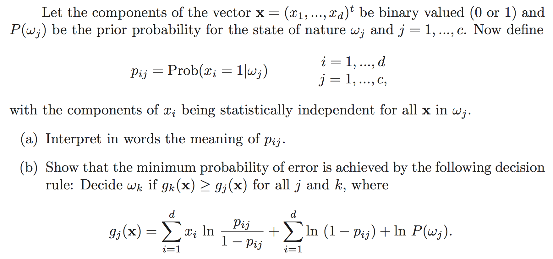
Let the components of the vector x = (x1,...,xd)t be binary valued (0 or 1) and P(ωj) be the prior probability for the state of nature ωj, j = 1,...,c. Define
pij = Prob(xi=1 | ωj), i = 1,...,d, j = 1,...,c,
with the components of xi being statistically independent for all x in ωj.
gj(x) = ∑i=1d xi ln (pij / (1−pij)) + ∑i=1d ln(1−pij) + ln P(ωj).
(Original problem statement, for reference: HW2_1.png.)
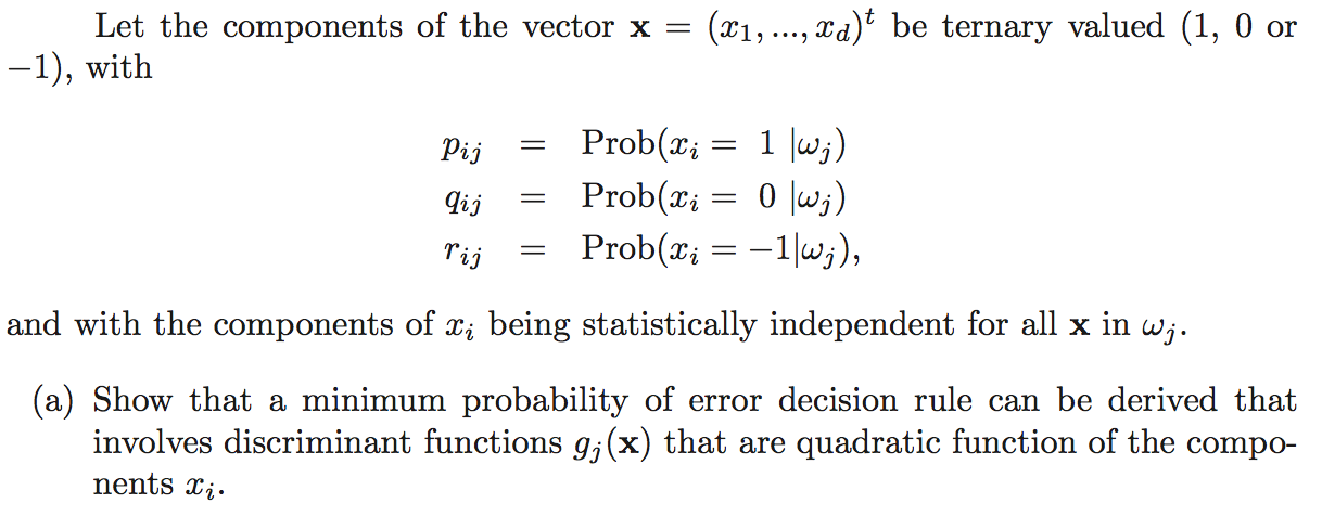
Let the components of the vector x = (x1,...,xd)t be ternary valued (1, 0, or −1), with
pij = Prob(xi=1 | ωj), qij = Prob(xi=0 | ωj), rij = Prob(xi=−1 | ωj),
and with the components of xi being statistically independent for all x in ωj.
A) Show that a minimum-probability-of-error decision rule can be derived that involves discriminant functions gj(x) that are quadratic functions of the components xi (contrast with Problem 13's binary case, where the discriminant was linear in x).
(Original problem statement, for reference: DHS_ch2_pb44_.png.)
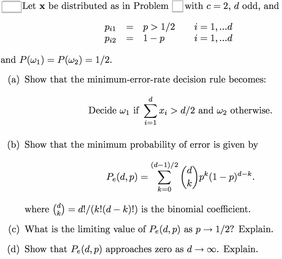
Builds on Problem 13. Let x be distributed as in Problem 13, with c=2, d odd, and
pi1 = p > 1/2, pi2 = 1−p, i = 1,...,d,
and P(ω1) = P(ω2) = 1/2.
Pe(d,p) = ∑k=0(d−1)/2 C(d,k) pk (1−p)d−k, where C(d,k) = d! / (k!(d−k)!).
(Original problem statement, for reference: DHS_ch2_pb45_.png.)
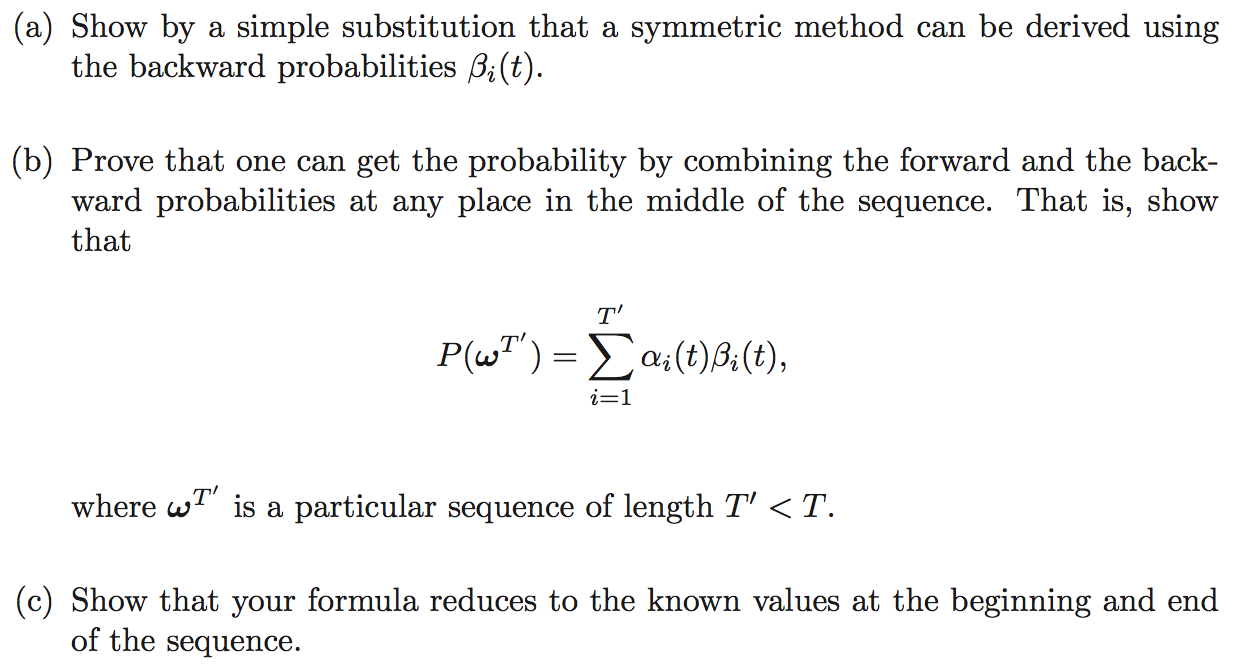
The standard method for computing the probability of a sequence in a given HMM uses the forward probabilities αi(t).
P(ωT') = ∑i=1T' αi(t) βi(t),
where ωT' is a particular sequence of length T' < T.
Note: the sum's index i runs over the N hidden states of the HMM (i.e. read the upper limit as N, not as the sequence length T' — the source problem statement uses the same symbol T' for both, which is a typo carried over from the original textbook printing).
(Original problem statement, for reference: HW3_1.png. Page 154–155 in DHS.)