Make sure you check the syllabus for the due date. Please use the notations adopted in class.
Instructions. Submit code (Jupyter notebook encouraged) plus a short report with tables and plots. Libraries (numpy, sklearn, matplotlib) are allowed for data handling, plotting, and basic math; the core algorithm of any "from scratch" problem must be your own. Several problems reuse your HW1 decision tree — keep it importable.
Note on normalization. When you normalize features (one feature at a time), normalize train, validation, and test together (using training statistics), not separately.
Requirements.
Datasets. Paths are relative to the course data folder (../../data/...). Core datasets: Housing (housing_train.txt / housing_test.txt, regression, pre-split) and Spambase (spambase/spambase.data, binary classification, one file — split 80/20 yourself). PROBLEM 3 uses the linearly-separable perceptron set (perceptronData.txt, 1000 points, 4 features + label ∈ {−1, +1}). The boosting stretch tier (PROBLEM 4) uses 8-class Newsgroups (or the full 20 Newsgroups).
Starter code. For each problem where a library counterpart exists, the starter notebook gives you the full data/eval pipeline and asks you to fill in two things: a short library-call baseline (a quick sanity-check number, using a well-known library function) and the from-scratch algorithm steps, evaluated the same way — your from-scratch number should land on or near the library one. Not every problem has a library counterpart to compare against (PROBLEM 5 is the one exception below); those are marked accordingly. Answers to the (THEORY) problems may be written directly in the notebook (e.g. a markdown cell) rather than a separate document, as long as they include any equation, plot, or illustration the answer depends on — not prose alone.
Implement batch gradient descent from scratch — you write the update rule and the loop yourself (no calling scipy.optimize or a library's own GD/SGD solver for the fit).
What's tested on Spambase: for both models, at one fixed threshold, a confusion matrix; and, sweeping the threshold across each model's own score range, a ROC curve with AUC — plot both models' ROC curves on the same axes so linear vs. logistic is a direct visual comparison.
Library sanity check: also fit sklearn.linear_model.Ridge (closed-form, same λ) for the linear model and sklearn.linear_model.LogisticRegression for the logistic model, on the same data, and report their train/test numbers alongside your from-scratch GD results — they should land in the same neighborhood (different solvers, same objective), not necessarily match exactly.
Library calls: sklearn.linear_model.Ridge, sklearn.linear_model.LogisticRegression.
On Spambase, fit L1-regularized (Lasso) regression across a range of penalty values (e.g. 20+ values of α spanning several orders of magnitude). A library implementation (sklearn.linear_model.Lasso) is allowed here — this problem is about the regularization path, not re-deriving Lasso's solver.
What's tested: for each α, threshold the prediction (as in PROBLEM 1) and record test accuracy, and count how many coefficients have been driven to exactly zero. Report two plots: (1) α vs. test accuracy, and (2) α vs. number of nonzero coefficients — together these should show the L1 penalty progressively eliminating features as α grows, and let you comment on where test performance starts to degrade as features are dropped.
Library calls: sklearn.linear_model.Lasso (this problem is library-only by design — there's no from-scratch counterpart required here; see PROBLEM 8 below if you want one).
Implement the perceptron mistake-driven update rule from scratch (initialize weights, and on each misclassified point nudge the weight vector toward the correct label) on the linearly-separable perceptron dataset (perceptronData.txt: 1000 points, 4 features + label ∈ {−1, +1}).
What's tested: a per-iteration mistake count, printed or plotted, that reaches 0 (this is guaranteed to happen — the data is linearly separable, so if your mistake count never reaches 0 you have a bug, not bad luck), and the final weight vector.
Library sanity check: also fit sklearn.linear_model.Perceptron on the same data. Since the data is linearly separable, both should reach 0 training errors — compare final decision boundaries (or the number of epochs/mistakes each needs to converge) between your version and the library's.
Library calls: sklearn.linear_model.Perceptron.
Now that you have logistic regression, boost for classification by gradient descent on the log-loss, reusing your HW1 regression tree as the weak learner (this is the one place in HW2 where the "from scratch" core must literally be your own earlier code, not a library tree):
[60 points] Core — Spambase (binary). Plot train/test error vs. number of rounds T — this should show the same overfitting-with-more-rounds story as HW1's boosted regression trees.
Library sanity check: also fit sklearn.ensemble.GradientBoostingClassifier (binary log-loss, matching tree depth and learning rate) on the same Spambase split, and plot its staged train/test error vs. round on the same axes as your from-scratch curve.
[+15 bonus points] Stretch — multiclass. Extend the same algorithm to multiclass: one accumulated score Fk(x) per class, softmax over classes instead of sigmoid, one weak learner fit per class per round. Run it on 8-class Newsgroups (or the full 20-class set) — same algorithm, harder data. A library tree (e.g. sklearn.tree.DecisionTreeRegressor) is fine for the weak learner here if your own from-scratch tree is too slow on high-dimensional text features.
Library sanity check (stretch): also fit sklearn.ensemble.GradientBoostingClassifier in its native multiclass mode on the same Newsgroups split, and report its accuracy alongside your from-scratch multiclass result.
Library calls: sklearn.ensemble.GradientBoostingClassifier (binary for the core tier, multiclass for the stretch tier).
Implement pool-based active learning by uncertainty sampling. Write one reusable loop (don't duplicate it per classifier): start from a small randomly-labeled seed set, train, reveal the true labels of the unlabeled points the current model is least certain about (closest to the decision boundary), add them to the training set, retrain, and repeat until the labeling budget is used up.
Run that same loop with two classifiers you already built above, both on Spambase:
What's tested: for each classifier, one plot of test accuracy vs. number of labeled points, overlaying an active-selection curve against a random-sampling baseline (same loop, but add random unlabeled points instead of the most-uncertain ones) — 2 plots total. Then, in a sentence or two, say which classifier benefits more from active selection and why (e.g. compare how large the gap over random sampling is, and at what point in the budget it appears).
Library calls: none — there's no standard library implementation of pool-based uncertainty sampling to compare against; the loop itself, built around classifiers you already have, is the from-scratch algorithm here.
Sweep the regularization strength λ for your PROBLEM 2 L1/Lasso fit and, separately, for an L2/ridge fit on the same data, plotting each feature's coefficient value against λ for both. As λ increases, L1 drives more and more coefficients to exactly zero (not just small), while L2 only ever shrinks coefficients smoothly toward (but not exactly to) zero. Meanwhile, test accuracy first improves, then declines as λ keeps increasing.
In a short written answer, explain, conceptually, why L1 regularization drives coefficients to exactly zero in a way that L2 does not, and explain why test accuracy eventually declines as λ keeps increasing.
Suppose two classifiers on the same test set achieve the identical AUC, but their ROC curves have very different shapes: one rises steeply at low false-positive rate (FPR) and levels off, while the other rises more gradually and evenly across the full FPR range. For a medical-screening-style application where missing a true positive is far more costly than a false alarm, and you need to pick a single operating threshold, propose which classifier you would choose and explain why AUC alone — being the same for both — does not tell you which is better for this specific use case.
PROBLEM 2 uses a library Lasso solver; this extends it — implement your own. Coordinate descent is the standard from-scratch approach here, since Lasso's L1 penalty isn't differentiable at 0 (which rules out plain gradient descent) but has a simple closed-form update one coordinate at a time.
For a fixed α, cycle repeatedly through coordinates j = 1..m, holding every other coefficient fixed, and at each step:
Repeat sweeps over all coordinates until θ stops changing (e.g. max coordinate change < 1e-6, or a fixed number of sweeps).
What's tested: run on Spambase (the PROBLEM 2 dataset) at a handful of α values spanning PROBLEM 2's sweep, and confirm your solver's coefficients (and the resulting test accuracy and nonzero-coefficient count) closely match sklearn.linear_model.Lasso at each α — here "closely" should mean genuinely close (both are solving the same convex objective to convergence), a tighter bar than PROBLEM 1's GD-vs-library sanity check.
Library calls: sklearn.linear_model.Lasso.
Replace PROBLEM 1's gradient-descent update for logistic regression with Newton-Raphson: at each step compute both the gradient and the Hessian of the log-likelihood at the current θ, and update θ ← θ − H−1∇ (instead of θ ← θ − η∇). Run it on Spambase and report train/test accuracy next to PROBLEM 1's GD result.
What's tested: the two should reach comparable accuracy, but Newton's method should converge in far fewer iterations (often single digits, vs. thousands for GD) since it uses local curvature instead of a fixed step size — report the iteration counts for both and comment on the difference.
Given a ranking of binary-labeled items by prediction score, the ROC curve plots true-positive rate against false-positive rate at every possible threshold, and the AUC is the area under that curve. Prove that the AUC also equals the fraction of item pairs (i, j) with different true labels that are ranked in the correct order (the positive-labeled item scores higher than the negative-labeled one).
Worked example to check your derivation against, before writing the general proof:
| object | score | true label |
| A | 100 | 1 |
| B | 99 | 1 |
| C | 96 | 0 |
| D | 95 | 1 |
| E | 90 | 1 |
| F | 85 | 0 |
| G | 82 | 1 |
| H | 60 | 0 |
| K | 40 | 0 |
| I | 38 | 0 |
The ROC curve comes from truncating this list at every rank and computing the false-positive-rate/true-positive-rate pair at that threshold. In this example, the item pairs in incorrect order are (C,D), (C,E), (C,G), (F,G) — use that to sanity-check whichever formula for AUC you end up deriving.
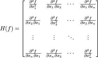
For a real-valued function f(x1,...,xn), the Hessian is the matrix of partial second derivatives:
Consider the log-likelihood function for logistic regression:

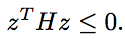
Show that its Hessian H is negative semidefinite, i.e. for any vector z:
This is sometimes written H ≼ 0, and implies the log-likelihood is concave — which is exactly why gradient ascent (or PROBLEM 9's Newton's method) on it has no spurious local optima to get stuck in.
Hint: 
Boosting extra-credit bank (each optional, no credit; PROBLEM 12's AdaBoost implementation is the base that PROBLEMS 13 and 18 build on).
Implement AdaBoost as described in class, using decision stumps (single feature/threshold splits) as the weak learner. For each feature: sort the training values, remove duplicates, and use the midpoints between successive values as candidate thresholds; a stump predicts +1 above its threshold and −1 below.
Run on Spambase, two ways:
What's tested: after each round, track (1) that round's own weighted stump error (should trend up toward 0.5 as rounds increase — the easy patterns get boosted away first), (2) train error and (3) test error of the combined classifier so far, and (4) test AUC. Report three plots (round error; train/test error; test AUC — all vs. round number) for each of the two stump-selection strategies, plus one final ROC curve on the test set to compare against PROBLEM 1's ROC curves.
Run your PROBLEM 12 AdaBoost on two more UCI datasets: CRX and VOTE (other UCI_simple sets are there too, if you want more comparisons). Each ships as a .config file (number of points; discrete/continuous attributes and, for discrete ones, their possible values; then the number of classes and their labels) and a .data file (one row per point, label last) — write a small parser for this format.
What's tested: for each of CRX and VOTE, train on c% of the data (chosen randomly), for c ∈ {5, 10, 15, 20, 30, 50, 80}, testing each time on the same fixed held-out fold; plot test accuracy vs. c. Repeat with a few different random training subsets (or cross-validate) if you want error bars on the curve.
Error-Correcting Output Codes (ECOC) are a stronger multiclass strategy than one-vs-rest: each of K ECOC functions splits the multiclass problem into one binary problem, so training gives you K independent binary AdaBoost models. At prediction time each of the K models outputs 0/1, producing a length-K "codeword"; the predicted class is whichever class's own codeword is closest (Hamming distance) to the observed one — see Dietterich & Bakiri's paper.
Run on 8-class Newsgroups (the original 20 labels, grouped into 8 to keep this tractable). The data is in sparse format: "label featureId:featureValue featureId:featureValue ..." — features not listed are exactly 0, not missing. Use either the exhaustive 127-function code from the paper above, or 20 randomly chosen ECOC functions; for each function, train AdaBoost with decision stumps for 200+ rounds.
Expected: this should take a few minutes and reach at least ~70% test accuracy.
Bag your HW1 decision tree: train T=50 trees from scratch, each on its own sample-with-replacement set drawn from the N-point training set (so some points repeat and others are left out of any given tree's sample) — you may cap tree depth to keep this fast. At test time, average the T trees' predictions.
What's tested: run on Spambase and compare test accuracy (and the train/test gap) against your PROBLEM 4 boosted-trees result. Bagging and boosting both combine many weak trees, but by very different mechanisms — i.i.d. resampling vs. sequential residual-fitting — comment on what you observe.
Implement RankBoost, following the RankBoost paper (Freund, Iyer, Schapire & Singer), and run it on the TREC 678 query set. This is a ranking task rather than a classification one: given a query, RankBoost learns to order documents by relevance rather than to classify each independently. Report whichever ranking metric the paper itself uses to evaluate the learned ranker.
Every boosting problem elsewhere in this HW works from a fixed, pre-extracted feature matrix. Here, extract features on the fly: at each boosting round, choose the next weak learner's feature based on the current per-point boosting weights, rather than fixing all features up front. Try this on (a) 20-Newsgroups raw text and (b) Digits/MNIST raw images — in each case, the feature-extraction step itself should depend on where the current ensemble is making mistakes.
Extend your PROBLEM 12 AdaBoost (decision stumps) with a feature-importance analysis: rank features by their share of the overall classifier's average margin — see the boosting-margin feature-analysis notes.
What's tested: run 300 rounds of AdaBoost on Spambase and report your top-10 features by this ranking. Then run the same analysis on polluted Spambase (same points, with extra noisy/duplicated columns injected) and check whether AdaBoost still identifies the real, informative features despite the added noise columns — and whether test accuracy holds up.
The lecture notes (see LOGREG_LOSS_claude_0910.pdf, “Feature Selection: Wrapper, Filter, and Embedded Methods”) describe three different families of feature-selection algorithm. PROBLEM 2 already gives you an embedded method (Lasso) for free; this problem asks you to build one method from each of the other two families and compare all three head to head, on the same data.
What's tested: report the three resulting top-10 feature sets side by side and how much they overlap with each other. Then retrain a simple classifier (e.g. logistic regression) using only each 10-feature subset in turn, and report test accuracy for all three — is any one family consistently better here, or do they land close to each other despite choosing different features and costing very different amounts of compute to run?
Library calls: sklearn.feature_selection.mutual_info_classif (filter), sklearn.linear_model.LogisticRegression (the fixed classifier used to score candidates during wrapper search and to evaluate all three final subsets). The wrapper's greedy search loop itself should be your own code, not SequentialFeatureSelector — the point is to see the retrain-every-step cost directly.