CS6140 Machine Learning — Fall 2026

HW3 — Kernels, SVM, Kernel Ridge, PCA, KPCA

Make sure you check the syllabus for the due date. Please use the notations adopted in class.

Instructions. Submit code (Jupyter notebook encouraged) plus a short report with tables and plots. Libraries (numpy, sklearn, matplotlib) are allowed for data handling, plotting, and basic math; the core of any "from scratch" problem must be your own.

Requirements.

• Fill in every TODO_STUDENT blank according to the algorithm steps covered in lecture and the linked materials, and make sure the notebook runs top to bottom without errors.
• Understand the whole notebook — including the provided/given code, not just the blanks you filled in — well enough to explain any part of it during office hours.

Model/hyperparameter selection. Wherever a problem asks you to choose among kernels, hyperparameters, or a dimension (Problem 1's kernel grid, Problem 2's kernel + regularization, Problem 4's T), split off a validation set and pick using validation performance only. Report the test-set number once, for the configuration you already chose — never pick a configuration by looking at test performance.

Reading. The lecture notes for this HW: PCA and Feature Representations, Kernels and Kernelized Algorithms, SVM with Kernels (optional: SVM, Advanced Topics, for the optional problems). Notation in the starter code follows these notes (e.g. the Gaussian kernel is exp(−‖x−z‖²/σ²), i.e. sklearn's gamma = 1/σ²). Dataset links in each problem are relative to the course data folder (../../data/...).

Starter code. For each problem where a library counterpart exists, the starter notebook gives you the full data/eval pipeline and asks you to fill in two things: a short library-call baseline (a quick sanity-check number, using a well-known library function) and the from-scratch algorithm steps, evaluated the same way — your from-scratch number should land on or near the library one. Answers to the (THEORY) problems may be written directly in the notebook (e.g. a markdown cell) rather than a separate document, as long as they include any equation, plot, or illustration the answer depends on — not prose alone.

PROBLEM 1 — SVM: library, then from scratch (Simplified SMO)   [100 points]

Parts A–B use an SVM library of your choice (e.g. LIBSVM, scikit-learn) on real data. Parts C–D implement your own SVM solver and check it against the same library.

• Part A (library, binary): Spambase. Try several kernels, including polynomial and RBF; report results.
• Part B (library, multiclass, required): the Digits/MNIST dataset (HAAR features). If your SVM package is binary only, write a multiclass wrapper — one-vs-the-rest (10 classifiers) or all-pairs voting (45 classifiers, predict by most wins).
• Part C (from scratch, linear kernel, correctness check): implement the Simplified SMO algorithm (SVM note, Section 5): iterate over all α_i, and whenever α_i violates the KKT conditions pick a random α_j among the rest and jointly optimize the pair. (The full Platt SMO adds an error cache and pair-selection heuristics for speed; it is optional Problem 8.) Write your solver so it only ever looks at a precomputed kernel (Gram) matrix, never raw features directly — that way the same code works for any kernel. Run it with a linear kernel on the TwoSpirals data (same file as Problem 4). Recover the primal weight vector w = ∑α_iy_ix_i and compare it against a library linear SVM's weight vector (e.g. SVC(kernel='linear').coef_) at the same C. They should match reasonably well — same direction and similar accuracy; an exact match also in magnitude needs full convergence, which the sweep cap may not reach on this non-separable data. Also compare the support vectors (your points with α_i>0 vs. the library's support_). This validates your optimizer even though a linear kernel classifies this data poorly (TwoSpirals is not linearly separable by construction).
• Part D (from scratch, RBF kernel, required): rerun the identical solver with an RBF Gram matrix in place of the linear one, on the same TwoSpirals train/test split. Compare accuracy against a library RBF-SVM on the same split — both should solve it almost perfectly, which is the actual point of the kernel trick (and of picking this dataset instead of Spambase, where Part A shows a linear kernel already does about as well as RBF).

Note: the "stop once a fixed number of sweeps pass with no change" stopping rule of the Simplified SMO algorithm is not guaranteed to trigger on noisy, non-separable data. Cap the total number of sweeps (e.g. 300) so your run time stays bounded regardless of whether that rule ever fires — without a cap this can run for a very long time.

Library calls: sklearn.svm.SVC (linear, polynomial and RBF kernels), sklearn.multiclass.OneVsRestClassifier.

PROBLEM 2 — Kernel Ridge Regression from scratch   [50 points]

Implement a kernel ridge regression wrapper with fit(X, y) and predict(X); the initializer selects the kernel (linear, polynomial, RBF) and its hyperparameters (regularization λ solved as α = (K + λI)^-1y; Kernels note, Section 8 — center the labels first, since this model has no intercept). The kernel evaluation may use a library, but the rest must be from scratch. Check your implementation against a library baseline (e.g. sklearn.kernel_ridge.KernelRidge) at the same kernel/hyperparameters.

• Fit the WAVE data (waveX, waveY) with linear, RBF, and polynomial kernels; tune hyperparameters on a validation split.
• Evaluate train/test MSE for each kernel and plot predicted vs true coordinates.
• Repeat for the CRESCENT data (crescentX, crescentY). Explain which kernel did better on each and why.

Library calls: sklearn.kernel_ridge.KernelRidge.

PROBLEM 3 — PCA from scratch (feature corruption & rescue)   [40 points]

Using the polluted Spambase dataset (original points, many extra junk / duplicated features):

• A) Train a classifier on the raw polluted features and observe the drop in performance relative to the same classifier on the original, unpolluted 57-feature Spambase — fit and report that unpolluted control inside this notebook, not just from memory of HW2's numbers (Spambase). Use logistic regression (from HW2) as the downstream classifier.
• B) Run PCA (a library is allowed here) to reduce to ~100 features, then retrain. Apply PCA consistently to train and test (fit on train, apply the stored transform to test). Explain the improvement.
• C) Implement your own PCA (PCA note, Section 6) and rerun the classifier on your PCA features.

Library calls: sklearn.decomposition.PCA, sklearn.linear_model.LogisticRegression.

PROBLEM 4 — Kernel PCA + linear classifier   [60 points]

Datasets: 1000 2-D points each — TwoSpirals (binary, chance ≈ 50%) and ThreeCircles (a balanced 3-class dataset despite the shared file format, chance ≈ 33%). Report chance level alongside accuracy so the two datasets' numbers aren't compared as if both were binary.

• A) Train a linear/logistic classifier and confirm it fails (high error, near chance) on the raw 2-D data.
• B) Run Kernel PCA with a Gaussian kernel (e.g. σ=1) to obtain a T-dimensional representation (build the kernel matrix, center it, eigendecompose, project — including the centering formula for new/test points; Kernels note, Section 11). Check your implementation against a library baseline (e.g. sklearn.decomposition.KernelPCA) at your chosen T.
• C) Retrain the linear classifier on the kernelized features, sweeping T over a few values (e.g. 2, 5, 10, 20, 50). Choose T on a validation split — e.g. the smallest T reaching some accuracy bar you define as "good" (such as 90% validation accuracy) — and confirm that choice once on the held-out test set. The two datasets are not equally hard, so don't expect the same T for both.

Library calls: sklearn.decomposition.KernelPCA, sklearn.linear_model.LogisticRegression.

PROBLEM 5 (THEORY) — Choosing the RBF Bandwidth in Kernel Ridge Regression   [25 points]

Fit your PROBLEM 2 kernel ridge regression on WAVE or CRESCENT with an RBF kernel at a very small bandwidth vs. a much larger bandwidth. With a very small bandwidth, the fitted curve passes almost exactly through every training point, with wild oscillations between them; with a larger bandwidth, it looks like a smooth curve that doesn't hit every point exactly, but tracks the overall trend.

In a short written answer, explain this pattern, and propose how to choose the bandwidth properly (i.e., not by eye and not by minimizing training error).

PROBLEM 6 (THEORY) — One-vs-Rest SVM Ambiguity in Multiclass Regions   [25 points]

Your PROBLEM 1 (Part B) one-vs-rest multiclass SVM wrapper trains one binary SVM per class and predicts using whichever classifier gives the most confident "positive" score. For most test points this works fine, but for points near the boundary between three or more classes, it is possible for all the binary classifiers to output a negative ("not this class") decision, leaving no clear winner — or, conversely, for multiple classifiers to claim the point positively.

In a short written answer, explain why one-vs-rest can produce this kind of ambiguous region, and propose whether switching to a one-vs-one (all-pairs) voting scheme would fix it.

Optional problems (no credit). Problems 7–10 have their own sections in the starter notebook: set RUN_OPTIONAL = True there to work on them. With the default False those cells are skipped, so the notebook still runs top to bottom.

PROBLEM 7 — t-SNE Dimensionality Reduction   [optional, no credit]

t-SNE isn't a kernel method, but it rhymes with this HW's PCA/KPCA problems: another way to turn high-dimensional data into something a 2-D plot (or a simple downstream classifier) can actually work with — and unlike PCA, it's built specifically to preserve local neighborhood structure, at the cost of not being a linear projection at all.

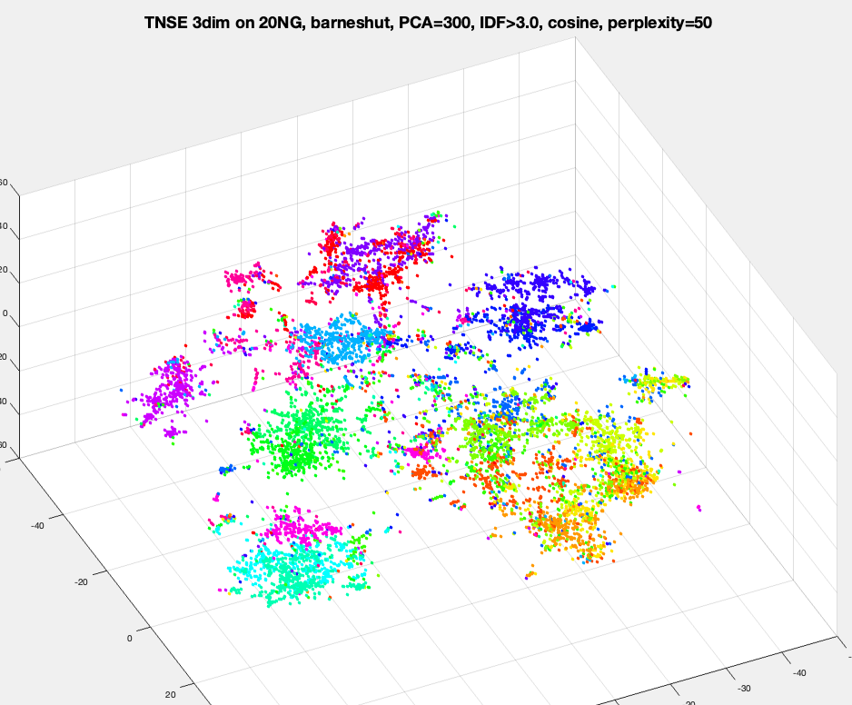
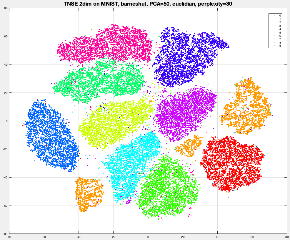
Part A (library). Run a library t-SNE (e.g. sklearn.manifold.TSNE) on MNIST and/or 20 Newsgroups, project to 2 or 3 dimensions, and scatter-plot the points colored by label. Try a few perplexity values (e.g. 5, 20, 100) and see how the picture changes. Here's what a good result looks like — each color is a different digit/newsgroup, and they should separate into fairly clean clusters:

Part B (from scratch, harder). Implement t-SNE yourself. We're deliberately not giving you code here — go read Laurens van der Maaten's own t-SNE page (the original author; it has the paper, reference implementations in several languages, and FAQ) and work from that. At a high level, the algorithm is:

1. Reduce the input to ~50 dimensions with PCA first (t-SNE itself is for refining local structure, not for crunching raw high-dimensional data efficiently).
2. Compute the pairwise squared-distance matrix in that reduced input space.
3. For each point i, binary-search a per-point bandwidth so the resulting conditional distribution over its neighbors has a fixed "effective number of neighbors" — matching a target perplexity via that distribution's entropy.
4. Symmetrize and normalize into one joint distribution P over all pairs, in the original high-dimensional space.
5. Initialize a random low-dimensional embedding Y; define Q as the (normalized) Student-t similarities between points in that embedding — the heavy tail is what gives t-SNE room to spread out clusters that would otherwise collapse on top of each other.
6. Gradient-descend (momentum/adaptive gains help a lot in practice) on KL(P ‖ Q), nudging points in Y until the low-dimensional similarities match the high-dimensional ones as well as they can.
7. Every few iterations, re-center Y and check in (plot it, watch the KL-divergence trend down) — this is as much art as it is algorithm.

Run your implementation on MNIST (or a manageable subsample of it) and compare your scatter plot against Part A's library result.

Library calls: sklearn.manifold.TSNE (Part A only — Part B is the from-scratch counterpart).

PROBLEM 8 — Four Ways to Reduce Dimensions: PCA, ICA, Kernel PCA, t-SNE   [optional, no credit]

Each method keeps something different: PCA keeps variance in uncorrelated directions, ICA looks for statistically independent components, Kernel PCA does PCA in a kernel feature space, and t-SNE keeps local neighborhoods. This problem shows a task where each objective matters (PCA note, optional ICA section; Kernels note, Section 11; Problem 7 for t-SNE).

• Part A (unmixing: where ICA wins). The "cocktail party" setup: generate 3 known source signals over time (e.g. a sine wave, a square wave, a sawtooth; 2000 time steps), mix them with a random 3×3 matrix A (each observed signal is a different blend of the three sources), then run PCA and ICA (sklearn.decomposition.FastICA) on the mixtures, keeping 3 components each. Plot the recovered components next to the true sources, and for each source report the largest |correlation| with any recovered component. Expected: PCA returns uncorrelated but still-mixed signals; ICA recovers the sources, up to order, sign and scale. Explain why: uncorrelated is not the same as independent, and PCA's directions are forced to be orthogonal while the columns of A need not be.
• Part B (embedding: where ICA has no particular advantage). On a digits/MNIST subsample (e.g. 2000 points of MNIST, or sklearn's small load_digits), standardize the features and reduce to 2-D with PCA, ICA, Kernel PCA (RBF), and t-SNE. Scatter-plot each embedding colored by label. Then split the embedded points into train/test (t-SNE has no transform for new points, so embed everything first) and report 5-NN accuracy on each 2-D embedding. Which keeps the class structure best, and why does t-SNE's local-neighborhood objective suit this task better than the variance (PCA) or independence (ICA) objectives?

Library calls: sklearn.decomposition.PCA, FastICA, KernelPCA, sklearn.manifold.TSNE, sklearn.neighbors.KNeighborsClassifier.

PROBLEM 9 — Random Fourier Features: Kernel Methods Without the N×N Matrix   [optional, no credit]

Kernel ridge regression stores and solves with an N×N matrix. Random Fourier features replace the Gaussian kernel with an explicit map z(x) of R random cosine features, so that z(x)z(x')^T ≈ K(x,x'); then plain (linear) ridge regression on z does the job (Kernels note, Section 14.3).

• Implement the map yourself: draw W with entries from N(0, 2/σ²) and phases b uniform on [0, 2π], and set z(x) = √(2/R) cos(xW + b). Check it: on a few hundred points, compare ZZ^T with the exact kernel matrix for R = 100, 1000, 10000 (the largest error should shrink roughly like 1/√R). Then check that sklearn's RBFSampler(gamma=1/σ²) behaves the same.
• On WAVE (waveX, waveY; same split as Problem 2), at your Problem 2 σ and λ: center y, fit ridge regression (no intercept) on z(x) for R ∈ {5, 10, 20, 50, 100, 300, 1000}, and plot test MSE against R, with your exact kernel ridge regression from Problem 2 as a horizontal line. Average over a few random seeds. Expected: a few dozen features already give a reasonable fit, and the gap to the exact kernel solution closes as R grows (about 1000 features to match it closely).
• [optional] Repeat with sklearn.kernel_approximation.Nystroem (M landmark points instead of R random features). On this 1-D dataset it should need far fewer components than random features. Why might that be? (Hint: look at how fast the eigenvalues of the kernel matrix decay.)

Library calls: sklearn.kernel_approximation.RBFSampler, Nystroem, sklearn.linear_model.Ridge, sklearn.kernel_ridge.KernelRidge.

PROBLEM 10 — Dr. Lawler's Patient Similarity: When a Similarity Is Not a Kernel   [optional, no credit]

Dr. Lawler, an endocrinologist, has compared patients the same way for years. On each of 6 routine lab tests, two patients "agree" if their values are within a clinical tolerance of each other, and "disagree" otherwise; a clear disagreement should count against similarity, so he scores +1 for agree and −1 for disagree, and averages over the tests:

s(a, b) = (1/6) ∑_k ( +1 if |a_k − b_k| ≤ t_k, −1 otherwise ),   with tolerances t = glucose 10 mg/dL, HbA1c 0.3 %, BMI 2, systolic BP 10 mmHg, LDL 15 mg/dL, triglycerides 30 mg/dL.

It is symmetric, between −1 and 1, and every patient is fully similar to themselves (s = 1), so it looks like a perfectly good similarity. After the kernel lectures he plugged it into Kernel PCA (to aggregate the 6 labs into a few features) and into an SVM with C = 10 (to predict who develops type-2 diabetes within 5 years), on 400 of his patients (lawler_patients.csv: patient id, the 6 labs, label diabetes_5yr; the data is synthetic). Things went wrong in strange ways. Help him.

• Part A (the symptoms). Build the 400×400 matrix S of his similarity.
  1. Kernel PCA. Run your Problem 4 Kernel PCA with K = S, but without dropping eigenvalues ≤ 0. Plot the eigenvalues ν of the centered matrix and report what fraction of the "variance" (the sum of all ν) the top T components explain, for T = 2, 10, 50, 100. What happens to the normalization β = u/√ν? Your Problem 4 code dropped eigenvalues ≤ 0 as "numerical noise" (Kernels note, Section 13). Is that what they are here?
  2. The margin. Train SVC(kernel='precomputed', C=10) on a 70/30 split. From its dual_coef_ (which holds α_iy_i for the support vectors) compute ‖w‖² = ∑_i,j α_iy_iα_jy_jS_ij (w = ∑α_iy_iΦ(x_i); SVM note, Sections 2 and 4) and the margin 1/‖w‖. What do you get?
  3. Same patients, different answers. Sort the training patients by glucose (as his spreadsheet happens to be), retrain with identical settings, and count how many test predictions change. Repeat over several random splits. Then run your own Problem 1 SMO solver on S with a few different random seeds: compare the final dual objectives and the predictions. With a valid kernel (e.g. the RBF kernel) none of this happens. Why not?
• Part B (the diagnosis). Look at three patients who differ only in glucose: 95, 105 and 115 mg/dL, using the glucose term alone. Write down their 3×3 similarity matrix and its eigenvalues. If a kernel K(a,b) = Φ(a)Φ(b)^T existed, the squared distance between two patients in feature space would be K(a,a) + K(b,b) − 2K(a,b). Compute it for the three pairs and explain in plain words why no feature map Φ can produce this matrix (hint: "A is like B and B is like C, but A is not like C"). Connect this to the "valid kernel ⇔ positive semidefinite" test in Kernels note, Section 3, and use it to explain each symptom of Part A: why can a real feature map never give a negative ‖w‖², and why does a non-PSD matrix give the SVM dual more than one "best" answer? Then find such a triple among his real patients.
• Part C (approximate fixes). Try three repairs and say what each one costs:
  1. Clip: eigendecompose S and set the negative eigenvalues to 0 (this is the closest positive semidefinite matrix). How much does S change (relative Frobenius norm)? Can you compute the clipped similarity between a new patient and the old ones?
  2. Shift: add |ν_min|·I to the training matrix. What does this do to the eigenvectors? Compare the size of the shift with the diagonal entries of S (which are 1). What do you expect the SVM to do with it?
  3. Soften: keep his idea of tolerances, but replace the hard +1/−1 window with a smooth bump, s'(a,b) = (1/6) ∑_k exp(−(a_k − b_k)²/t_k²). Explain why this one is a valid kernel (Kernels note, Sections 3–4: a Gaussian kernel on one feature, and a sum of valid kernels), and check its eigenvalues.
• Part D (does it matter?). Predict diabetes_5yr with SVC(kernel='precomputed') using his raw S at his C = 10, then with C chosen on a validation split for each of: raw S, clipped, shifted, softened, and a standard RBF kernel on standardized labs. Clip and shift the training block only; evaluate the test rows with the raw similarities. Average the test accuracy over several random splits, and compare with the majority-class rate. Which would you recommend to Dr. Lawler, and why?

What to expect: nearly half of the eigenvalues are negative and large, so the "variance explained" goes well above 100% and β turns into NaNs; ‖w‖² comes out negative, so the margin is not a number; reordering the patients changes on the order of 10% of the predictions (sometimes far more), and different SMO seeds stop at different objectives. In Part D not every repair helps: one of them collapses to predicting "no diabetes" for everyone. The softened similarity is the one he can actually use, including for new patients.

Library calls: numpy.linalg.eigh, sklearn.svm.SVC(kernel='precomputed'), sklearn.model_selection.train_test_split.

PROBLEM 11 — SVM-SMO on the Digits Dataset   [optional, no credit]

Instead of a library SVM, run your own Problem 1 SMO solver on the Digits dataset. Digits has 10 classes and your SMO is a binary classifier, so you need a multiclass wrapper on top of it — choose one of:

• One-vs-the-rest: train 10 binary SMO classifiers, one per class.
• ECOC on top of SMO: same idea as ECOC boosting, just with your SMO solver as the base binary classifier.
• All-pairs voting: train all (10 choose 2) = 45 one-vs-one models (e.g. the "7 vs 9" model trains/tests only on points labeled 7 or 9). At test time, run all 45 models and predict the class with the most wins; break ties using the direct head-to-head match.

Digits is learnable enough that you can subsample the training set (e.g. 10–20% per class) to keep runtime down — but evaluate on the full test set.

PROBLEM 12 — The Full Platt SMO Algorithm   [optional, no credit]

Problem 1 (Parts C–D) uses the CS229 Simplified SMO algorithm (random second-variable selection, no error cache). Extra credit for implementing the full Platt SMO heuristics instead, following the Platt SMO paper (summary in the SVM Advanced note, Section 6):

• a maintained error cache, so you're not recomputing E_i from scratch for every point on every sweep;
• the entire-set / non-bound-subset alternation (sweep all points, then only the non-bound ones, alternating until neither changes anything);
• the second-choice heuristic for picking α_j — maximize |E_i − E_j| among non-bound points first, falling back to a scan over the non-bound set and then the full set if that makes no progress (instead of Problem 1's uniform-random pick).

Reference implementations already exist in this course's materials (6_SVM_kernels/code_HW6/bingyu/SVM/SVM.py, SMO.java) if you want to check your work against them — but implement your own rather than copying them.

PROBLEM 13 — Solve the Dual with a Library QP Solver   [optional, no credit]

Same problem as Problem 1, Parts C–D, but instead of SMO, solve the SVM dual directly with a general-purpose quadratic-programming solver (e.g. cvxopt.solvers.qp in Python, or an equivalent in Matlab/Java/C); the SVM Advanced note, Section 5, writes the dual in the matrix form these solvers expect. Compare the resulting α's and accuracy against your SMO solution.

PROBLEM 14 — Six-Point Hyperplane by Inspection   [optional, no credit]

Consider the following 6 points in 2-D, for two classes:

class 0:   (1,1)   (2,2)   (2,0)
class 1:   (0,0)   (1,0)   (0,1)

a) Plot these 6 points, construct the optimal hyperplane by inspection and intuition (give W, b) and calculate the margin.
b) Which points are support vectors?
c) [Extra credit] Construct the hyperplane by solving the dual optimization problem using the Lagrangian. Compare with part (a).

PROBLEM 15 — The Dual Constraint 0 ≤ α ≤ C/m   [optional, no credit]

Explain why 0 ≤ α ≤ C/m is a constraint in the dual optimization with slack variables (hint: read the Burges SVM tutorial first). Distinguish three cases, and explain each in terms of the classification and the constraints: a) α = 0; b) 0 < α < C/m; c) α = C/m. This has been discussed in class and in the SVM notes (SVM note, Section 3; SVM Advanced note, Sections 2–3); a detailed, rigorous explanation is expected, not just a restatement of the three cases.

PROBLEM 16 — VC Dimension   [optional, no credit]

What is the VC dimension of an SVM with a linear kernel? (Mostly of historical interest; see the last section of the SVM Advanced note.)

PROBLEM 17 — LDA Instead of PCA   [optional, no credit]

Problem 3 rescues polluted Spambase with PCA. Run LDA instead of PCA before the downstream logistic regression classifier — you can use a library LDA implementation (e.g. sklearn.discriminant_analysis.LinearDiscriminantAnalysis; Fisher's LDA is in the optional part of the PCA note). Compare accuracy against Problem 3's PCA result.

PROBLEM 18 — DHS Chapter 5   [optional, no credit]

Pick a problem from DHS (Duda, Hart & Stork, Pattern Classification) chapter 5 (linear discriminant functions / SVMs) that isn't already covered above, and solve it. If you're not sure which one to pick, ask.

PROBLEM 19 — Linear SVM by Subgradient Descent (Pegasos)   [optional, no credit]

The soft-margin SVM is also an unconstrained problem: a regularizer plus the average hinge loss, (λ/2)‖w‖² + (1/N)∑_i max(0, 1 − y_i(x_iw + b)), with λ = 1/(NC) (SVM Advanced note, Section 7). That means it can be trained like HW2's logistic regression, one point at a time, with no dual and no kernel matrix.

• Implement Pegasos (the algorithm box in SVM Advanced note, Section 7): pick a random training point, step size η_t = 1/(λt), shrink w, and push it toward y_ix_i only if that point is inside the margin or misclassified. Fold the intercept in with a constant feature x⁰ = 1.
• Run it on standardized Spambase (same split as Problem 1 Part A) at the C that Part A selected for the linear kernel. Plot the objective and the test accuracy against the number of passes over the data (e.g. up to 30).
• Compare with LinearSVC / SVC(kernel='linear') at the same C: final objective, test accuracy, and the cosine similarity between the two weight vectors. Expected: after about 30 passes, Pegasos reaches the same test accuracy and a weight vector with cosine similarity ≈ 0.99 (an exact match needs many more steps; for larger C, i.e. smaller λ, convergence is slower).
• In a few sentences: how does the Pegasos update differ from the perceptron update (HW2), and which part of it produces the large margin?

Library calls: sklearn.svm.LinearSVC, sklearn.svm.SVC (sklearn.linear_model.SGDClassifier(loss='hinge') is the library version of the same idea).

PROBLEM 20 — Support Vector Regression vs. Kernel Ridge Regression   [optional, no credit]

SVR replaces the hinge with the ε-insensitive loss: residuals smaller than ε cost nothing, so all points inside a tube of half-width ε around the fit get zero weight (SVM Advanced note, Section 8). Kernel ridge regression (Problem 2) gives every training point a weight.

• On WAVE (waveX, waveY; same split as Problem 2), fit sklearn.svm.SVR with an RBF kernel at the σ your Problem 2 selected (gamma = 1/σ²), for ε ∈ {0, 0.05, 0.1, 0.2, 0.3}, choosing C on the validation set for each ε.
• Report a table: ε, chosen C, test MSE, and the number of support vectors (len(model.support_)), next to your Problem 2 kernel ridge regression (test MSE, and how many of its weights α_i are nonzero).
• Plot the fit with its ε-tube and circle the support vectors for two values of ε. Expected: around ε ≈ 0.1–0.2 (about the noise level of WAVE) SVR matches kernel ridge regression's test MSE using a small fraction of the training points; ε = 0 uses all of them; too large an ε flattens the fit.

Library calls: sklearn.svm.SVR, sklearn.kernel_ridge.KernelRidge.