CS6140 Machine Learning

HW4 Boosting, Features, PCA, Active Learning, ECOC

Make sure you check the syllabus for the due date. Please use the notations adopted in class, even if the problem is stated in the book using a different notation.

In this HW you can use libraries (such as sklearn) for training Decision Trees, one-hot encoding / data preprocessing, and other math functions.

Make sure you check the syllabus for the due date. Please use the notations adopted in class, even if the problem is stated in the book using a different notation.

SpamBase-Polluted dataset: the same datapoints as in the original Spambase dataset, only with a lot more columns (features) : either random values, or somewhat loose features, or duplicated original features.

SpamBase-Polluted with missing values dataset: train, test. Same dataset, except some values (picked at random) have been deleted.

Digits Dataset (Training data, labels. Testing data, labels): about 60,000 images, each 28x28 pixels representing digit scans. Each image is labeled with the digit represented, one of 10 classes: 0,1,2,...,9.

PROBLEM 1 [50p] Gradient Boosted Trees for Regression

Run gradient boosting with regression trees on housing dataset. Essentially repeat the following procedure i=1:10 rounds on the training set. Start in round i=1with labels Y_x as the original labels.

Train a regression tree T_i of depth 2 on data X, labels Y_x (use your HW1 regression tree code as a procedure, or use a library).
Update labels for each datapoint x : Y_x = Y_x - T_i(x). No need to update a distribution over datapoints like in Adaboost.
Repeat

The overall prediction function is the sum of the trees. Report training and testing error as a. function of T = number of trees in the ensemble

PROBLEM 2 [50p] Gradient Boosted Trees for classification

Run gradient boosting with regression stumps/trees on 20Newsgroup dataset dataset. Or you can use 20Newsgroup_8classes dataset with extracted features (The zip file is called 8newsgroup.zip because the 20 labels have been grouped into 8 classes to make the problem easier). Or you can download 20NewsGroup from scikit-learn

PROBLEM 3 L1 Feature Selection [50 points]

Run a strongL1-regularized regression (library) on 20NG dataset 8-class version, and select 200 features (words) based on regression coefficients absolute value.
Then reconstruct the dateaset with only these selected features, and run L2-regularized classifier (library). Report accuracy per class.

PROBLEM 4 PCA features [50 points]

Spambase polluted dataset.
A) Train and test Naive Bayes. Why the dramatic decrease in performance ? Expected Accuracy with Gaussian Fits: 62%

B) Run PCA first on the dataset in order to reduce dimensionality to about 100 features. You can use a PCA package or library of your choice.
Then train/test Naive Bayes on the PCA features. Explain the performance improvement. (To make it work, you have to apply PCA consistently to training and testing points: either apply for training and store the PCA transformation to apply it later for each test point; or apply PCA once for entire dataset)
Expected Accuracy on Naive Bayes with Gaussian Fits, running on PCA features: 73%.

C) Implement your own PCA, and rerun Naive Bayes on obtained features.

D) [Optional , no credit] Run LDA instead of PCA before you train the Naive Bayes. You can use a LDA package or library of your choice.

PROBLEM 5 PCA features for images [50 points]

Mnist Digit Dataset or Mnist (plain text) Digit Dataset Hint: For extracting the MNIST dataset, here are example code for Python, MATLAB Java
Run PCA to reduce dimensionality of the dataset to 30 features. The train and test a Grad Boosted Tree with 10 scoring functions (one per class) and report performance.

PROBLEM 6 [Optional, no credit] Error Correcting Output Codes

Run Boosting with ECOC functions on the 20Newsgroup dataset with extracted features. The zip file is called 8newsgroup.zip because the 20 labels have been grouped into 8 classes to make the problem easier. The features are unigram counts, preselected by us to keep only the relevant ones.

There are no missing values here! The dataset is written in a SPARSE FORMAT: "label featureId:featureValue featureId:featureValue featureId:featureValue ...". The features not listed are not missing values, they have zero values which were not written down to save space. In a full-matrix format, these values would be 0.

ECOC are a better multiclass approach than one-vs-the-rest. Each ECOC function partition the multiclass dataset into two labels; then Boosting runs binary. Having K ECOC functions means having K binary boosting models. On prediction, each of the K models predicts 0/1 and so the prediction is a "codeword" of length K 11000110101... from which the actual class have to be identified.

You can use the following setup for 20newsgroup data set.

- Use the exhaustive codes with 127 ECOC functions as described in the ECOC paper, or randomly select 20 functions.

- Use all the given features

- For each ECOC function, train an AdaBoost with decision stumps for 200 or more iterations

The above procedure takes a few minutes (Cheng's optimized code, running on a Haswell i5 laptop) and gives us at least 70% accuracy on the test set.

PROBLEM 7 Adaboost code [Optional, no credit]

Implement the boosting algorithm as described in class. Note that the specification of boosting provides a clean interface between boosting (the meta-learner) and the underlying weak learning algorithm: in each round, boosting provides a weighted data set to the weak learner, and the weak learner provides a predictor in return. You may choose to keep this clean interface (which would allow you to run boosting over most any weak learner) or you may choose to more simply incorporate the weak learning algorithm inside your boosting code.

Decision Stumps as simple classifiers

Each predictor will correspond to a decision stump, which is just a feature-threshold pair (f,t); in other words a single-split decision tree. Note that for each feature, you may have many possible thresholds which we shall denote . Given an instance, a decision stump predict +1 if the input instance has a feature value exceeding the threshold otherwise, it predicts -1. To create the various thresholds for each feature you should

sort the training examples by their f_i values
remove duplicate values, and
construct thresholds that are midway between successive feature values.

Boosting with Decision Stumps

Run your Adaboost code on the Spambase dataset

"Optimal" Decision Stumps: Run your implementation of boosting with "optimal" decision stumps on the training data. After each round, you should compute (1) the local "round" error for the decision stump returned, (2) the current training error for the weighted linear combination predictor at this round, (3) the current testing error for the weighted linear combination predictor at this round, and (4) the current test AUC for the weighted linear combination predictor at this round.
- Create three plots: One for the local "round" error (which should go up as rounds increase), one for the training and test error (which should both go down as rounds increase), and one for the test AUC (which should go up as the rounds increase). You should boost until you see "convergence" in test error or AUC.
- For the final weighted linear combination that is produced, create an ROC curve on the test data and compare your results to those you obtained in previous assignments.
You should think carefully about how you can efficiently generate the required results above. For example, I would suggest keeping a running weighted linear prediction value (before thresholding at zero) for each training and testing instance: when each new round predictor is created, you can simply update your running weighted linear prediction value and then easily compute training and testing error rates (by thresholding these values at zero), as well as testing AUCs (by ranking the instances by these values).
"Randomly Chosen" Decision Stumps: Repeat the procedure above for "randomly chosen" decision stumps. Note that you will almost certainly have to boost for more rounds to "converge".

PROBLEM 8 [Optional, no credit] Adaboost on UCI datasets

UCI datasets: AGR, BAL, BAND, CAR, CMC, CRX, MONK, NUR, TIC, VOTE. (These are archives which I downloaded a while ago. For more details and more datasets visit http://archive.ics.uci.edu/ml/). The relevant files in each folder are only two:
   * .config : # of datapoints, number of discrete attributes, # of continuous (numeric) attributes. For the discrete ones, the possible values are provided, in order, one line for each attribute. The next line in the config file is the number of classes and their labels.
    * .data: following the .config convention the datapoints are listed, last column are the class labels.
You should write a parser that given the .config file, reads the data from the .data file.

A. Run the Adaboost code on the UCI data and report the results. The datasets CRX, VOTE are required, rest are optional

B. Run the algorithm for each of the required datasets using c% of the datapoints chosen randomly for training, for several c values: 5, 10, 15, 20, 30, 50, 80. Test on a fixed fold (not used for training). For statistical significance, you can repeat the experiment with different randomly selected data or you can use cross-validation.

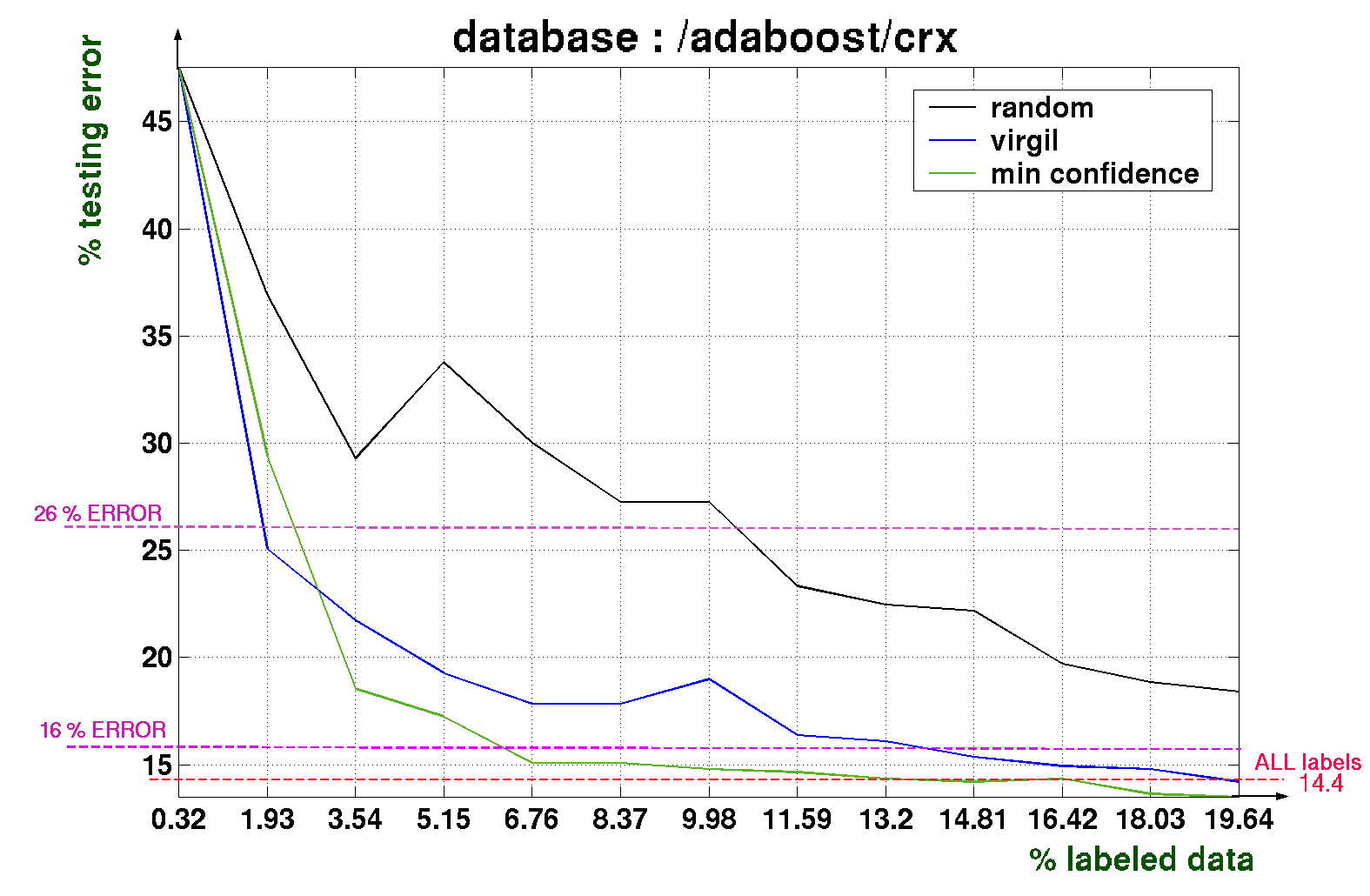
C: Active Learning Run your code from PB1 on Spambase, CRX, VOTE dataset to perform Active Learning. Specifically:

- start with a training set of about 5% of the data (selected randomly)

- iterate: train the Adaboost for T rounds; from the datapoints not in the training set; select the 2.5% ones that are closest to the separation surface (boosting score F(x) closest to 0) and add these to the training set (with labels). Keep training the ensemble, every T boosting rounds add data to training set until the size of the training set reaches 60% of the data.

How is the performance improving with the training set increase? Compare the performance of the Adaboost algorithm on the c% randomly selected training set with c% actively-built training set for several values of c : 5, 10, 15, 20, 30, 50. Perhaps you can obtain results like these

PROBLEM 9 Missing Values [Optional, no credit]

A) Spambase polluted dataset with missing values: train, test. Run a slightly modified Naive Bayes to deal with the missing values, as described in notes following KMurphy 8.6.2. (Essentially runs the independence product from Naive Bayes ignoring the factors corresponding to missing features.)
Expected Accuracy when using Bernoulli fits: 80%.

B) [Optional no credit] Run tSNE library first on the dataset, computing distances/similarities with missing values. Then re-train and test Naive Bayes using the tSNE representations.

PROBLEM 10 [Optional, no credit] Bagging

Bagging setup:

Training: Run your Decision Tree classifier separately (from scratch) T=50 times. Each Decision Tree is trained on a sample-with-replacement set from the training dataset (every Decision Tree has its own sampled-training-set). You can limit the depth of the tree in order to simplify computation.

Sampling with replacement: Say there are N datapoints in the training set. Sampling with replacement, uniformly, for a sample of size N, works in the following way: in a sequence, independently of each other, select randomly and uniformly N times from the training datapoints. Once a datapoint is selected, it is still available for further sampling (hence "with replacement" methodology). Each sampled-training-set will have N datapoints; some points will be sampled overall more than once (duplicates) while other datapoints will not be sampled at all.

Testing: for a test datapoint, will run all T Decision Trees and average the predictions to obtain the final prediction.

Run bagging on Spambase dataset. Compare results with boosting.

PROBLEM 11 [optional, no credit]

Run Boosting with ECOC functions on the Letter Recognition Data Set (also a multiclass dataset).

PROBLEM 12 [optional, no credit] Boosted Decision Trees

Do PB1 with weak learners being full decision trees instead of stumps. The final classifier is referred as "boosted trees". Compare the results. Hints: there are two possible ways of doing this.

Option 1. The weights are taken into account when we decide the best split, like in Adaboost. This requires you to change the decision tree training : when looking for best split at each node, the split criteria has to account for current datapoints weights as assigned by the boosting.

Option 2. We can simulate the weights by sampling. In each round, when we want to train the decision tree, we construct a new data set based on the old one. We sample from the old data set k times with replacement. In each sampling, each data point x_i in the old data set has probability w_i of being chosen into the new data set. k can be as large as the size old data set, or smaller. We only need to make sure there are enough data points sampled for a decision tree to be trained reliably. Then we train a decision tree on the new data set without considering weights. Weights are already considered in sampling. In this way, you don't need to modify the decision tree training algorithm. More generally, any weak learner, whether it can handle weights naturally or not, can be trained like this. Once the decision tree is trained, the new data set is discarded. The only use of the newly constructed data set is in building the tree. Any other computation is based on the original data set.

PROBLEM 13 [optional, no credit] Rankboost

- Implement rankboost algorithm following the rankboost paper and run it on TREC queries.

PROBLEM 14 Boosting with Dynamic Features [Optional, no credit]

A) Run Boosting (Adaboost or Rankboost or Gradient Boosting) to text documents from 20 Newsgroups without extracting features in advance. Extract features for each round of boosting based on current boosting weights.

B) Run Boosting (Adaboost or Rankboost or Gradient Boosting) to image datapoints from Digit Dataset without extracting features in advance. Extract features for each round of boosting based on current boosting weights. You can follow this paper.

PROBLEM 15 [Optional, no credit] Adaboost with bad features

A) Spambase (original dataset) : Implement feature analysis for Adaboost as part of your boosting code. Run Adaboost with Decision Stumps for 300 rounds; then list the top ten features : rank features by the fraction of average margin (of the overall classifier) due to each feature.
Cheng's top 15 features (IDs as column number in data, starting at 0): 52, 51, 56, 15, 6, 22, 23, 4, 26, 24, 7, 54, 5, 19, 18.

B) Spambase polluted dataset : Run Adaboost on polluted Spambase and report performance - why does it still work? Expected Accuracy: 93%.

PROBLEM 16 [Optional, no credit] Regularized Regression for noise data

A) Spambase polluted dataset run Logistic Regression for classification. Expected Accuracy: 85%

B) Run Regularized Regression (separate runs for LASSO and RIDGE) using a package for regularization. For example use the scikit-learn (Python) or Liblinear (C++) implementation of LASSO. Compare with Logistic Regression performance. Expected Accuracy of Lasso Logistic Regression: 93%.

C) Implement your own RIDGE optimization for Logistic Regression. Expected Accuracy of Ridge Logistic Regression: 92%.

D) Implement your own LASSO optimization for linear regression.

PROBLEM 17 Image Feature Extraction [Optional, no credit]

Mnist Digit Dataset or Mnist (plain text) Digit Dataset

Implement and run HAAR feature Extraction for each image on the Digit Dataset. Then train and test a 10-class ECOC-Boosting on the extracted features and report performance. You can sample the training set (say 20% of each class), in order to scale down the computation.
Expected Accuracy when using 200 HAAR features, 50 random ECOC, each Adaboost trained for 200 rounds: 89%.

(Hint: For extracting the MNIST dataset, here are example code for Python, MATLAB Java )

HAAR features for Digits Dataset :First randomly select/generate 100 rectangles fitting inside 28x28 image box. A good idea (not mandatory) is to make rectangle be constrained to have approx 130-170 area, which implies each side should be at least 5. The set of rectangles is fixed for all images. For each image, extract two HAAR features per rectangle (total 200 features):

the black horizontal difference black(left-half) - black(right-half)
the black vertical difference black(top-half) - black(bottom-half)

You will need to implement efficiently a method to compute the black amount (number of pixels) in a rectangle, essentially a procedure black(rectangle). Make sure you follow the idea presented in notes : first compute all black (rectangle OBCD) with O fixed corner of an image. These O-cornered rectangles can be computed efficiently with dynamic programming
black(rectangle OBCD)= black(rectangle-diag(OD)) = count of black points in OBCD matrix
for i=rows
for j=columns
black(rectangle-diag(OD_ij)) = black(rectangle-diag(OD_i,j-1)) + black(rectangle-diag(OD_i-1,j))
- black(rectangle-diag(OD_i-1,j-1)) + black(pixel D_ij)
end for
end for

Assuming all such rectangles cornered at O have their black computed and stored, the procedure for general rectangles is quite easy:
black(rectangle ABCD) = black(OTYD) - black(OTXB) - black(OZYC) + black(OZXA)

The last step is to compute the two feature (horizontal, vertical) values as differences:
vertical_feature_value(rectangle ABCD) = black(ABQR) - black(QRCD)
horizontal_feature_value(rectangle ABCD) = black(AMCN) - black(MBND)