Make sure you check the syllabus for the due date. Please use the notations adopted in class.
Where this HW sits. HW1–HW4 used numpy/sklearn and built classical models by hand. From here on the model is a neural network and the tool is PyTorch (with the d2l book's helpers). The comparison runs the other way now: you first build a network from scratch in numpy (Problems 1–2), and then check it against the same network in PyTorch. After that, PyTorch carries the core (the second half of Problem 2, and Problem 3), and you build only the specific mechanism each part is about: inverted dropout, the VAE's reparameterization and KL term. Problem 4's GAN is complete code that you run, read, and explain.
Setup. HW5–HW7 share one environment (PyTorch + d2l). Follow the NN setup page before starting. Every problem in this HW runs on a laptop CPU.
Instructions. Submit code (Jupyter notebook encouraged) plus a short report with tables and plots. Libraries (numpy, matplotlib, torch, torchvision, d2l) are allowed for data handling, plotting, and standard layers. Where a problem or part says "from scratch", the forward pass, the backward pass (gradients), and the update rule must be your own numpy code: no torch, no autograd.
Requirements.
Datasets. Paths are relative to the course data folder (../../data/...). Wine (train / test, 3 classes, 13 features; Problem 2, for fast debugging). Fashion-MNIST (28×28 grayscale clothing images, 10 classes, 60,000 train / 10,000 test; downloaded automatically into the course data folder (../../data/torchvision/) by torchvision.datasets.FashionMNIST, the same data d2l.FashionMNIST wraps; Problem 2) — the d2l book's standard dataset, and the one HW6's CNNs start from, so your MLP numbers here become the baseline for them. MNIST (handwritten digits, same format; downloaded automatically by torchvision.datasets.MNIST; Problem 3). 2-D Gaussian mixtures 2gaussian.txt / 3gaussian.txt, the same toy data as HW4 Problem 3 (Problem 4).
Starter code. The starter notebook gives you the device cell, data loading, plotting, a small train-and-log helper, and a checkpoint cell after each piece you implement. A checkpoint cell runs a provided test (a gradient check, or a comparison against the matching PyTorch function), so you know a piece is correct before you build on it. For each from-scratch part, the starter asks for both your implementation and the matching PyTorch version, evaluated the same way; the two numbers should land on or near each other. Answers to the (THEORY) problems, and to written parts inside other problems, may be written directly in the notebook (e.g. a markdown cell) rather than a separate document, as long as they include any equation, plot, or illustration the answer depends on — not prose alone.
Consider a neural network with 8 input units, 3 hidden units, and 8 output units, all with sigmoid activations, trained on the 8 one-hot inputs below, where each target output equals its input:
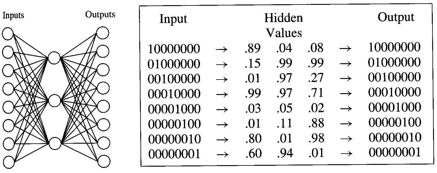
This is a tiny network, so the point is how you build it: the same way PyTorch does, as a chain of layers, each of which knows its own forward and backward pass (d2l 5.3).
(A — 15 points) Layers with forward and backward. Implement three numpy classes: Linear (weights W and bias b), Sigmoid, and SquareLoss. Each has forward(x), which returns the output and caches whatever the backward pass will need, and backward(grad_out), which returns the gradient with respect to its input (and, for Linear, also stores dL/dW and dL/db). The network is a list of layers: forward runs the list in order, backward runs it in reverse, passing each layer's returned gradient to the layer before it. That reverse loop is backpropagation.
(B — 15 points) Check the gradients, two ways. Before training, verify every gradient:
Fix any failure before you continue: a network trained on wrong gradients can still look like it is learning.
(C — 20 points) Train it, and read what it learned. Train with gradient descent from nontrivial random initial weights (not values that already minimize the error). Plot the loss vs. iteration, and report the table of hidden-unit values for the 8 inputs. You should obtain values similar to the table above, up to a permutation of hidden units and of 0/1 roles. Document any implementation choices (learning rate, number of iterations). Then, in a short written answer: since the outputs equal the inputs, this network is an encoder-decoder. What does training achieve in this context, and why is the 3-unit hidden layer (rather than, say, 8 units) essential to that? (Hint: round the hidden values to 0/1.)
Library calls: torch.nn.Linear, torch.nn.Sigmoid, torch.nn.MSELoss, torch.Tensor.backward.
The central problem of this HW. In Part I you build a multiclass network three ways: from scratch, with the wrong loss, and in PyTorch. In Part II you take the PyTorch version and study the training choices that decide whether a network learns well, learns badly, or doesn't learn at all. The starter's train-and-log helper makes each Part II run a few lines, so the work there is in setting up the comparisons and reading the plots.
Part I — Build it. Classification with a network means a softmax output layer trained with cross-entropy (maximum likelihood), the same objective as HW2's logistic regression, now with hidden layers in front of it. See d2l 4.4 and d2l 5.2.
(A — 25 points, from scratch) Extend your Problem 1 layer library with a ReLU layer and a combined SoftmaxCrossEntropy loss layer. Its backward pass is simply softmax(o) − onehot(y): see Equation 4 of the Basics note (§5.2), derived in §2 of the Advanced note. Compute softmax stably by subtracting max(o) before exponentiating. Add minibatch SGD. Then:
(B — 10 points) Why cross-entropy? Retrain the Fashion-MNIST network with Problem 1's recipe instead: sigmoid outputs and square loss against one-hot targets, with the same learning rate and budget of epochs. Plot both loss curves (or test accuracy vs. epoch) on one figure. In 2–3 sentences, explain the difference using the output-layer gradient: compare the softmax/cross-entropy gradient from (A) with what the sigmoid's derivative does to the square-loss gradient when an output is confidently wrong.
(C — 15 points, using PyTorch / d2l) Build the same 784–256–10 architecture as a d2l Module (nn.Flatten, nn.Linear, nn.ReLU, nn.Linear) and train it with d2l.Trainer (or the plain PyTorch loop on the setup page) using the same optimizer settings. Report a table of train/test accuracy for your from-scratch network and the PyTorch one, on both Wine and Fashion-MNIST. They should agree to within a percent or two. If they don't, the difference is a bug (the learning rate, the initialization scale, and softmax averaging vs. summing over the batch are the usual suspects).
Part II — Train it well. Everything from here on is in PyTorch, starting from (C)'s network.
(D — 15 points) Optimizers and the learning rate. Train the same network with: plain SGD at three learning rates (e.g. 0.01, 0.1, 1.0); SGD with momentum 0.9; and Adam (lr=10−3). Plot training loss vs. iteration for all five on one figure, and report final test accuracy in a table. Problem 6 builds on these curves. See d2l 12.6 (momentum) and d2l 12.10 (Adam).
(E — 20 points) Regularization: weight decay and dropout. To make overfitting visible, train the starter's wider network (with Adam) on a 5,000-image subset of Fashion-MNIST, long enough that training accuracy is clearly above test accuracy. Then:
Plot train and test accuracy vs. epoch for no regularization, your best weight decay, and dropout; report the final train/test gap for each. Problem 5 asks you to explain what you see.
(F — 15 points) Initialization and vanishing gradients. Build a 10-hidden-layer MLP (width 128) in four variants: {sigmoid, ReLU} activations × {small fixed-scale init, e.g. N(0, 0.012), the scaled init matched to the activation (Xavier for sigmoid, He/Kaiming for ReLU)}. For each, run one forward and backward pass on one batch and plot the gradient norm of each layer's weights, from the first layer to the last (log scale). Then train each variant briefly: which ones learn at all? In 2–3 sentences, connect the plot to the chain rule you implemented in Problem 1: what happens to a product of many per-layer factors that are each smaller than 1? (HW6's batch normalization and residual connections, and the LSTM's gates, are three designs aimed at exactly this problem.) See d2l 5.4.
Library calls: torch.nn.Linear, torch.nn.ReLU, torch.nn.CrossEntropyLoss, d2l.Trainer (Part I); torch.optim.SGD, torch.optim.Adam, torch.nn.Dropout, torch.nn.init.xavier_uniform_, torch.nn.init.kaiming_uniform_ (Part II).
See Lecture notes: Variational Autoencoders. Problem 1's autoencoder learns to compress and reconstruct, but nothing organizes its latent codes, and there is no principled way to generate a new point: you would have to guess a latent vector and hope the decoder produces something meaningful. A VAE makes the latent space a probability distribution shaped like a simple prior N(0, I), and that is what makes sampling and interpolation meaningful. Data: MNIST, flattened to 784 pixel values in [0,1].
Structurally, this is less new than it sounds. The decoder is the same "stack of Linear + activation" recipe as Problem 1's decoder half. The only new architectural piece is an encoder with two output heads (one for μ, one for logσ²) sharing one trunk. See the lecture note's "How new is this, structurally?" section.
(A — 20 points) Build and train it.
(B — 15 points) Explore the latent space. Three views of what the VAE learned:
(C — 15 points, written only) In HW4 Problem 3(C), you identified q(z|x) and p(z) for a Gaussian mixture fit with EM, where q(z|x) (the responsibilities) is computed exactly at every E-step. This VAE optimizes the same evidence lower bound (ELBO), but its q(z|x) is the encoder network from part (A), trained by gradient descent rather than computed in closed form. Explain why EM's E-step can be computed exactly for a Gaussian mixture but not for this VAE's decoder, and why a learned encoder is the right fix (rather than, say, just running more EM iterations).
Library calls: torch.nn.Linear, torch.nn.functional.binary_cross_entropy, torch.distributions.Normal (for the Monte-Carlo checkpoint), torchvision.datasets.MNIST. There is no standard library VAE to compare against; the checkpoints and the pictures in (B) are the validation.
See Lecture notes: GANs and d2l 20.1. HW4 Problem 3 fit a Gaussian mixture by writing down a likelihood and maximizing it; Problem 3 above maximizes a lower bound on one. A GAN takes a third approach and never writes down a density at all. The code for this problem is complete: the starter gives you both networks (a 2-D-noise → 2-D-point generator G, and a 2-D-point → score discriminator D), the alternating training step, and the plots. Your job is to run the experiments below, read the training step until you can explain every line of it, and answer the questions from what you see.
(A — 5 points) Two modes: how a GAN trains. Run the GAN on (standardized) 2gaussian.txt. The starter shows real vs. generated points at steps 0, 500, 2000, 4000, and D's and G's losses vs. step. Answer:
(B — 5 points) Three modes: when a GAN fails. Run the same GAN on 3gaussian.txt under three provided schedules: the default (1 D step per G step), G 5× stronger (5 G steps per D step), and D 5× stronger (5 D steps per G step). For each, the starter plots the final samples and prints the fraction of samples nearest each true mode and each mode's spread, next to the real data's. Answer: what happens under each schedule? Use the numbers, not just the pictures: a mode can have the right share of points but the wrong shape. Explain the mechanism of mode collapse in terms of what G is rewarded for. Finally, compare with HW4's EM fit of the same data, which is far less prone to this failure: why? (See the lecture note's "Common Failure Modes".)
Library calls: none to write. The provided code uses torch.nn.BCEWithLogitsLoss and torch.optim.Adam.
In Problem 2(E), adding dropout most likely lowered your training accuracy, raised (or held) your test accuracy, and shrank the train/test gap. (If your run didn't show this clearly, say so and explain why your setup might not show it.)
In a short written answer, explain why dropout produces this pattern. Then explain (conceptually) why dropout is turned off at test time rather than left on, and what the 1/(1−p) scaling in your inverted-dropout implementation is for.
Two students train the same network with gradient descent and plot training loss vs. iteration. Student A's curve decreases for a few iterations, then starts oscillating wildly and trending upward. Student B's curve decreases smoothly but extremely slowly, flattening out after many iterations at a loss still far above what a properly-tuned run achieves.
In a short written answer, diagnose each student's problem in terms of the learning rate and explain the mechanism behind each pattern (not just "it's too big/small"; think of the step size relative to the curvature of the loss). Point to which of your own Problem 2(D) curves, if any, look like A's or B's.
A third student, C, trains with minibatch SGD. C's curve drops quickly, then settles into a band that keeps jittering up and down, and it gets no narrower or lower even when C trains ten times longer. Nothing diverges, and C's loss evaluated once per epoch on the whole training set is smooth. Where does the jitter come from? (It is not the curvature story above.) Name two changes that would let C's loss settle lower, and what each one costs. Which of your raw Problem 2(D) curves show a band like this?
Follow d2l 20.2 (DCGAN) to generate Fashion-MNIST images, reusing Problem 4's training step unchanged. Only G and D change, from MLPs to (transposed-)convolutional networks. This previews HW6's convolutions.
For Problem 2's network (one ReLU hidden layer, softmax output, cross-entropy loss, a minibatch X of n examples), derive dL/dW2, dL/db2, dL/dW1, dL/db1 as matrix expressions (no sums over examples or units), and check that they match what your layer classes compute. A worked derivation of the max-likelihood (cross-entropy) output layer: notes.