Ridge Regression1
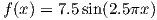
Conisder the polynomial regression task, where the task is to fit a polynomial of a pre-chosen degree to a sample of data comprising of data sampled from the function:
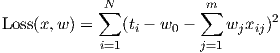
to which some random noise is added. So that the training labels can be represented as:
 | (1) |
where ϵ ~ Normal(0,σ2) is additive Gaussian noise. The training dataset  is therefore represented as
(xi,ti) ∀i ∈{1,2,…N}.
is therefore represented as
(xi,ti) ∀i ∈{1,2,…N}.
Figure-2 shows an example of fitting a degree-1 (straight line) and degree-3 (cubic polynomial), to a training dataset comprising of eight instances. It can be seen in Figure-1a that if we use a degree-1 polynomial as our hypothesis class we are unable to represent the function accurately, it is very intuitive because as compared to the target function our chosen hypothesis class is very simple. This is an example of underfitting where the hypothesis class fails to capture the complexities of the target concept. Figure-3a shows that a higher order polynomial (degree-6 in this case) fails to accurately represent the target function even though it perfectly predicts the label of each training instance. This is an example of overfitting, where instead of learning the target concept the learned concept aligns itself with the idiosyncrasies (noise) of the observed data. On the other hand by using a cubic polynomial (Figure-1b), we can see that it better rerepsents the target function, while having a higher training error than the degree-6 polynomial.
What happens when we overfit to the training data? Figure-3b, shows that in the case of overfitting, we achieve lower training errors but the error on unseen data (test error) is higher. So, what can we do to avoid overfitting? We have previously seen that in the case of Decision trees, we used pre-pruning and post-pruning to obtain shorter/simpler trees. Preferring simpler hypotheses that may have higher training error, over more complex hypotheses that have lower training error is an example of Occam’s Razor. William of Occam was an English friar and philosopher who put forward this principle which states that “if one can explain a phenomenon without assuming this or that hypothetical entity, then there is no ground for assuming it i.e. that one should always opt for an explanation in terms of the fewest possible number of causes, factors, or variables”. In terms of machine learning this simply implies that we should always prefer the simplest hypothesis that fits our training data, because “simpler hypothesis generalize well”.
How can we apply Occam’s Razor to linear regression? In other words, how can we characterize the complexity of linear regression? Recall, that in the case of decision trees the model complexity was represented by the depth of the tree. A shorter tree therefore, corresponded to a simpler hypothesis. For linear regression, the model complexity is associated with the number of features. As the number of features grow, the model becomes more complex, and is able to capture local structure in data (compare the three plots for the polynomial regression example in Figures 2 and 4), this results in high variance of estimates for feature coefficients i.e., wi. This means that small changes in the training data will cause large changes in the final coefficient estimates. In order to to apply Occam’s razor to linear regression we need to restrict/constrain the feature coefficients.
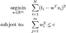
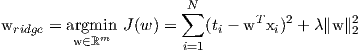
For linear regression, we can impose a constraint on the feature coefficients so that we penalize the solutions that produce larger estimates. This can be achieved by augmenting the original linear regression objective with a constraint as follows:
 | (2) |
The objective function is exactly the same as before for linear regression: minimize the sum of squares errors over the training data. However, we have an added constraint on the feature weights that restricts them form growing abnormally large. By formulating the Lagrangian of Equation-2 we get the following optimization problem:
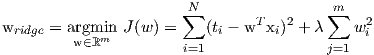 | (3) |
for λ ≥ 0. There is a one-to-one correspondence between λ and c in Equation 2. For a two dimensional case i.e., w ∈ ℝ2, we can visualize the optimization problem as shown in Figure-5.

We know, that:
therefore, we can re-write the problem as:
 | (4) |
Including an L2 penalty term in the optimization problem is also known as Tirkhonov regularization.
We can get an analytical solution similar to how we derived the normal equations. Before we proceed we need to address the fact that the intercept or w0 is part of the weight vector that we are optimizing. If we place a constraint on w0 then essentially our solution will change if we re-scale the ti’s. By convention, we are going to drop the constant feature (all ones) from the design matrix, and also center each feature i.e., subtract the mean from the feature values. Let Z be the centered data matrix and let t be the vector of observed target values (generated according to Equation 1).
Then,
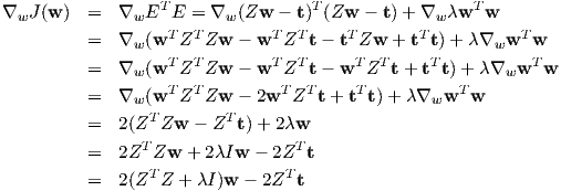
Setting the derivative to zero, we obtain

This solution corresponds to a particular λ, which is a hyper-parameter that we have chosen before hand. Algorithm-1 shows the steps involved in estimating the ridge regression solution for a given training set.
 ∑
i=1Nti;
∑
i=1Nti; ridge = (ZT Z + λI)-1ZT t;
Algorithm 1: The gradient descent algorithm for minimizing a function.
ridge = (ZT Z + λI)-1ZT t;
Algorithm 1: The gradient descent algorithm for minimizing a function.
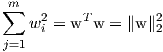
We can cast the objective function of ridge regression into a more general framework as follows:
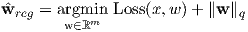
where, q represents the qth vector norm. Some of the regularizers corresponding to different values of q are shown in Figure-6. The loss function for Ridge regression (for centered features) is given as: