CSU540 Computer Graphics - Fall 2005 - Last three topics

Last three topics - Will be on Final Exam

CSU540 Computer Graphics - Fall 2005 - Prof. Futrelle

Updated 5 December 2005

Version with Phong shading, posted Sat Dec 3 20:30h EST 2005

Version with BSP tree, posted Sat Dec 3 21:55h EST 2005

Version with antialising, posted Sun Dec 4 16:35h EST 2005

Addtional material on BSP trees posted Mon Dec 5 05:15h EST 2005

As I said in class, we will go over three simple topics (or at least, simple versions of them). They are

Phong vertex-based shading for highlights
BSP trees (binary space partitioning trees)
Antialiasing

Each of these is treated in turn below.

Phong vertex-based shading for highlights

As the book explains in Sec. 9.2 (through 9.2.2), there are two approaches to Phong shading, both dealing with highlights related to the relation of the eyepoint direction e and the reflected ray direction r.

The basic Phong term that is added to the diffuse and ambient terms of pg. 193, is the one in eq. 9.5: c = c_l (e•r)^p, where I've omitted the max function, which is not critical to understanding the basic idea. The equation can also be viewed as stating that the Phong contribution to the illumination is proportional to (cosφ)^p, where φ is the angle between the eye direction and the reflected ray.

The first technique, which is the simplest Phong shading, interpolates the illumination across each triangle, just as Gouraud shading does, but it takes into account the (partial) specular behavior of the surface. This technique can be described as follows:

Find the normals for each triangle

Find the average of the normals of all the triangles surrounding each vertex.

Compute the illumination at each vertex using these average normals, using the additional Phong illumination term described above, applied to each of the three vertices. The diffuse and ambient terms are used in addition to the Phong term.

Interpolate the illumination across each triangle, e.g., by using barycentric coordinates.

For ray tracing the above, a hit would yield the barycentric coordinates for the hit value. Those coordinates would be applied to interpolate the illumination values based on the values already computed at the three vertices.

The second technique, Phong normal interpolation, described in Sec. 9.2.2, first interpolates the normals across the triangles, and then computes the illumination for each interpolated normal. In detail:

Find the normals for each triangle

Find the average of the normals of all the triangles surrounding each vertex.

Interpolate the normals across the triangle, e.g., by using barycentric coordinates.

For each interpolated normal value, compute the illumination as before using the Phong term, equation 9.5 in addition to the diffuse and ambient terms.

For ray tracing the above, a hit would yield the barycentric coordinates for the hit value. Those coordinates would be applied to interpolate the normal values based on the normals already computed at the three vertices.

For the given hit point the illumination is computed as in step d.

What you'll need to be able to do for Phong shading on the Final

You need to be able to write out the full illumination equation as of sum of the three terms for diffuse, ambient, and Phong illumination.

You need to be able to compute and make a sketch of cosφ, (cosφ)², (cosφ)⁴, using a few values for cosφ I'll give you, e.g., 1/2, 1/3.

You need to be able to explain how normal vector interpolation is done and draw a rough sketch to illustrate it.

BSP trees (binary space partitioning trees)

Here's the cool BSP applet site that's important for your Final Exam: http://symbolcraft.com/graphics/bsp/

The BSP tree is an important strategy in real-time graphics, because it involves one up-front computation for (unchanging) scene elements which can then be rapidly rendered from any viewpoint. The essence of the technique depends on using the painter's algorithm (Fig. 8.1), which consists of painting items farthest from the viewpoint first, then closer ones, with the closer ones possibly occluding the ones rendered earlier in the sequence. This automatically eliminates hidden surfaces. The scene is divided by planes. A tree is built. When a ray from the viewpoint strikes the plane at the root of the tree, it strikes it from one side or another. Items on the farther side are rendered first. While working on that half of the tree, each node is again examined, and whichever children of that node that are on the farther side are also rendered first, and so forth. The cool applet site I discovered shows this clearly, after some study.

The question you'll be asked on the Final about BSP trees will depend entirely on your already having experimented with the applet so you have a good understanding of the relation between the positions of planes in space, the corresponding tree structure, and what it implies for rendering order. Also, some objects may be bisected, even more than once by another plane, creating additional partial planes and corresponding nodes. Here are some of the types of experiments you can do with the applet to help your understanding, always starting with the simplest possible experiments.

Begin with a series of experiments with only two planes (represented as lines in 2D in the top boxes). You'll notice that each plane is oriented, with a normal projecting from it. Note that drawing a plane vertical and upwards orients it to the right, and vice versa when drawn vertically downward.

Move your lines and the viewpoint around, seeing how the tree changes.

For each vantage point you choose, figure out the painter's algorithm order and compare it to the tree and to the orientation of the planes in the tree.

Then create examples with three or four planes and do further experiments. Finally, recreate the example in the figure below and do similar experiments.

It's important to realize that in the simple demo as in our textbook that planes are being placed with respect to other planes. So the objects themselves are used as the partitioning surfaces. In some treatments of BSP trees, the planes and objects are quite distinct; not in our case.

Walking the tree: This be seen in the example figure below, where the tree walk is explained in addition. The traversal algorithm is presented in pseudocode on page 180 of the text. But in the figure below, the strategy becomes clear. The recursive traversal algorithm, in its simplest possible form is the following:

draw(tree, eyepoint){
  If tree empty: return;
  Choose the appropriate subtree and draw(subtree, eyepoint);
  Draw the root triangle;
  Choose the otherSubtree and draw(otherSubtree, eyepoint);
  }

The example screenshot and its intuitive trace/explanation

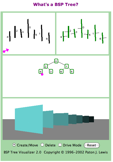First, note carefully how the tree is constructed. The first plane drawn is 0. The next is 1, drawn on the backside of 0, as related to 0's normal, so it is in a right subtree. Note that in the subtree under 1, node 5 is on 1's backside, so it is in the right subtree of 1. 6 is on the frontside of 1, the side that 1's normal projects to, so it is placed in 1's left subtree.
Exactly the same rules apply to the left subtree of 0, the subtree on 0's frontside. Once node 2 is created, 3 is in its right subtree, because it is on 2's backside, just as 5 is on the backside of 1. Node 4 is on the frontside of 2 so it forms the left subtree of 2.
Now for the traversal of the tree. The eyepoint is on the positive side of the root node 0, so we examine the subtree that is further away, the tree on 0's backside, the tree with 1, 5, and 6. These will be the ones drawn first. We draw the tree rooted at 1. Since the eyepoint is on the backside of 1, we follow the tree away from the eyepoint, the tree on the 1's frontside, which is 6. Since 6 has no subtrees, we return and draw 6. When we return to node 1, we know that the remaining subtree is closer to the eyepoint, so we draw node 1 and traverse subtree 5.
We then return to node 0 and draw that, since its left tree contains objects closer to the eyepoint. We then examine the 2 subtree. 2 faces the eyepoint, so we pursue the tree on the opposite face which is 3. After drawing that, 2 is drawn and the other subtree, 4, is entered and 4 is drawn.
Collecting all drawing operations above together, we see that the sequence of drawing is 6, 1, 5, 0, 3, 2, and 4, as it must be to render the scene correctly.
NB: If you open the image on the left in a separate window, you'll see it in more detail..

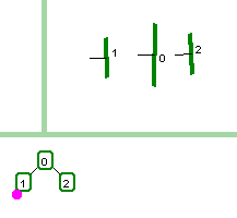
Two simple screenshots that show how the position with respect to the frontside and backside of a surface determine which subtree an object will be placed in.


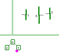
The key to understanding the placement of objects in the tree is to pay attention to the orientation of the partitioning surfaces. In the example above, the initial plane, 0, is drawn with its positive normal to the left. Then plane 1 is positioned on the positive side of 0 so it is placed in the left, positive, subtree of 0.	In the above example, plane 0 is oriented to the right. When plane 1 is drawn in the same location as before it is now on the backside of 0, so it is in the right subtree. Plane 2, on the positive or frontside of 0, is in the left, positive subtree of 0.

In each case, the viewpoint (not shown) was placed at the lower left corner, oriented up and to the right. This accounts for the pink circles in the trees, corresponding to the viewpoint. In either case, when viewing is done, the key to tree traversal is to see which side of each subtree root node the vector from the viewpoint/eyepoint strikes the plane corresponding to that node. Once that's determined, the subtree farthest from the viewpoint is drawn first.

What you'll need to be able to do for BSP trees on the Final

Basically, you will be given a screenshot similar to, but simpler than the example just described. It will only show you the top two boxes, not including the tree.

You will then have to construct the tree.

Finally, you will need to describe how the tree is traversed to give you the drawing order that will be obvious from the screenshot.

Antialiasing

Antialiasing is the simplest of the three topics. You'll need to know the basics of oversampling and also "jittering". The simple basics are covered in your textbook in Sec. 3.7. Jittering, usually called stratified sampling, is covered in Sec. 10.11.1. Both sections are short. What's not shown clearly is what I've illustrated in the figure below.

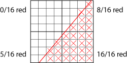
In the figure, the value in a single pixel can be estimated by rendering an area in a high-resolution array and then downsampling by averaging values. The figure below shows the computations done to render four pixels. Each pixel is represented by a 4x4 portion of a large array. The red region is rendered in the large array with its "pixels" marked as red or background (white in this case). By counting the small pixels, an estimate can be made about the proportion of red that should be rendered in each of the four actual pixels that will appear in the final image. For example, the lower left pixel is 5/16 red and 11/16 background. Since red can be represented as 255,0,0, and white as 255,255,255, this would yield a light red color of 255,175,175 (because 11/16 of 255 is about 175). Another way to think of this light red color is to realize that it is composed of 175,175,175 (a light, colorless gray) plus 80,0,0, a modest but pure red component.

What you'll need to be able to do for antialiasing on the Final

You'll need to be able to do two things: (1) Create a sketch such as in the figure above and compute (estimate) RGB values for it. (2) Draw diagrams such as in Figs. 10.27, 10.28, and 10.29 and explain why they illustrate different strategies for sampling. In the 4x4 strategy in the figure above, you should imagine that the sampling was done by regular or jittered samples. If it had been done by random samples, some of the pixels might have been missed entirely and some weighted more than once.

Go to CSU540 home page. or RPF's Teaching Gateway or homepage