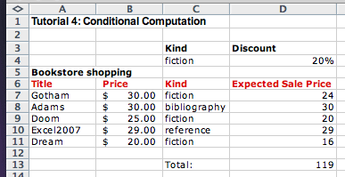
At times the result of a computation depends on whether some condition has been satisfied. For example, our favorite bookstore may sell fiction books at a 20% discount. We want to compute the total price of the purchase of several books. Here is what our calculations should look like:

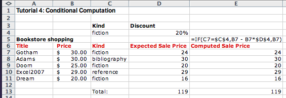
How can we compute the sale price, if the computation depends on whether the book is a fiction? The following function performs the desired conditional computation for the first row:
=IF(C7=$C$4,B7 - B7*$D$4,B7)
We compare the values of the cell C7 and the fixed cell
C4 to determine whether this book is a fiction book. The
next two arguments for the IF function define the two
possible actions; the first action is taken if the condition is
TRUE, the second is taken if the condition is
FALSE. We can now drag the formula down to compute the
sale price for each book:
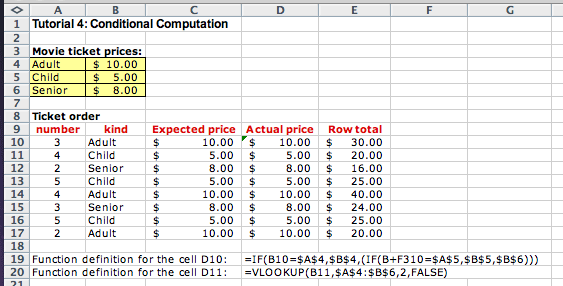
We now have a more complicated decision to make. We are selling tickets for a movie theater and there are three kinds of prices: a regular price for adults, and two different discounted prices for seniors and children. We make a table that shows the categories and the prices:

We now want to compute the amount the cashier takes in as the ticket sales are being made. A sample sequence of ticket purchases is shown here, together with the expected outcomes:
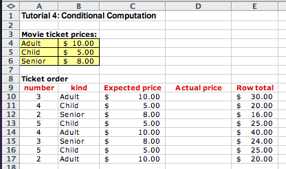
We can compute the desired price by a complicated formula that asks two IF questions as follows:
=IF(B10=$A$4,$B$4,(IF(B10=$A$5,$B$5,$B$6)))
to compute the price in the cell D10. While this may work
fine for just three categories, it becomes terribly cumbersome and
confusing when we are faced with several different
categories. Instead, we use the VLOOKUP function. When
you want to insert the VLOOKUP function it is the best to
go through the Insert menu so that your selection of the
function arguments is guided by a dialog box.
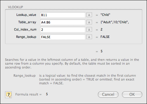
We want to look up the ticket kind in the cell B11 and
look up a matching value in the first column of the range of the
lookup data A4:B6. Once we find the value, we place in
the current cell the corresponding value from the column 2 of the
lookup data. In our case this is the column that gives us the
corresponding prices. If we place this VLOOKUP function
in the cell D11 we will produce the desired price for a
single Child ticket. However, if we try to drag the formula
down to the cells D12 through D17 it will
not work. We forgot to fix the reference for the lookup data
range. Here is the final table:
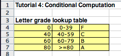
We now work out a similar problem where the lookup values are numerical values that may not match exactly our lookup table. For example, the instructor wants to assign letter grades to students based on the number of points earned on homeworks and exams. We start by setting up a lookup table:
Because the values we are trying to match are not exact, we omit the
last argument to the VLOOKUP function. Notice that the
dialog explains how this argument works:
It also reminds us that the values in the first column must be sorted in ascending order. Fortunately, we did this correctly. The value in our cell is compared to the values in the lookup table. To match, our value must be larger than or equal to the lookup value and smaller than the next entry in the lookup table. (For the last category, all values larger than the last value match that category.)
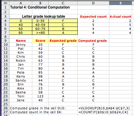
Let us now use this table to assign grades to the following students:
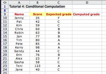
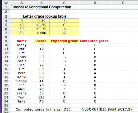
We use the VLOOKUP function as shown:
We now want to count how many As, Bs, Cs, and Fs did the students
earn. Another function COUNTIF helps us in this task. We
add a count column to the original lookup table. We compute the first
value as
=COUNTIF(D10:D24,C7)
However, we cannot drag this formula unless we fix the range of data to which we refer. So the correct formula is:
=COUNTIF($D$10:$D$24,C7)
and we get:
Practice these skills and explore the Excel behavior on the following problems: