There is a large number of standard mathematical functions used in business, statistical, scientific, and other modeling applications. One of the nice features of the Excel application is that it defines the computation for over 100 different functions and allows the user to use them by just selecting the appropriate function from one of the menus and provide the function with the appropriate arguments.
When you decide to use one of these functions, your first responsibility is to understand the computation the function performs. In most cases you should be able to compute simple examples of these function by hand or by looking up a bit of information about the underlying computation.
We will look at some of these functions to illustrate the variety of situations to which they can be applied. We will start with showing a step-by-step process that allows you to understand the underlying computation and design your program systematically.
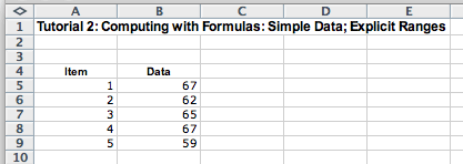
We start with a spreadsheet that shows five data values and the item number for each:

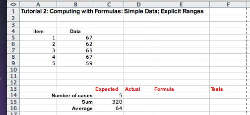
We would like to compute the average of these five values. To do so, we need to compute the sum of five items and to divide the sum by the number of items we have (which is five). We do this on a simple example where we can calculate the expected results by hand - and then verify that the computation/program we designed does indeed produce the same results. It is important that you can always show on a small example (or examples) what the expected result will be and that you verify at the end that your solution indeed produces the expected results.
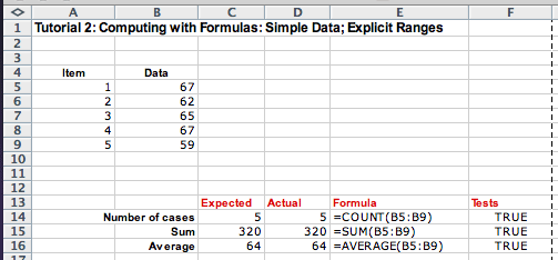
Here are our expected results. We set up a column for computing the results using Excel built-in formulas, showing the formulas we have used, and a column for tests where we compare the expected value with the actual computed value:
Functions over Ranges: Both expected values, the number of cases and the sum, require that we process a whole list of values. There are only five values in our list, but we would like to do a similar computation for lists of 100, or even 1000 data items.
Excel provides functions that consume a list of data and produce a
result based on the values in the whole list. The list of data we use
is called range and is specified by its first and last
cell with a : between the two cell references. In our
case, it is B5:B9. The three functions that consume a range
of data that perform the desired computation are COUNT,
SUM, and AVERAGE:
We can define a name for a range of data by selecting the Name Manager inside of the Formula menu bar. We can assign a name to the range and specify the cells it contains. We can include several lists of data in one range, for example, the range (B3:B7, B9:B13, B15:19) represents 15 data items in column B, in rows 3 through 19 with rows 8, and 14 omitted.
We define the range called DataRange that represents the
cells B5:B9, and use it in the functions MEDIAN,
MEAN, MAXIMUM, and MINIMUM:
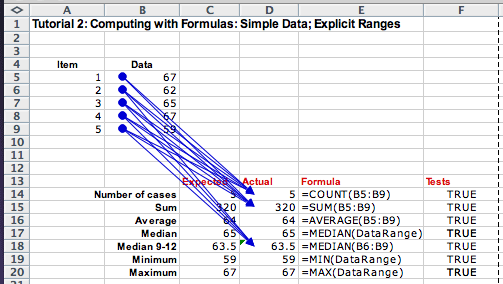
We have included here the arrows that show the dependents of the cells B5 through B9. You can add these arrows to your program by selecting the Trace Dependents inside of the Formula menu bar. Similarly, you can see what cells provide the inputs for your computation by selecting the Trace Precedents inside of the Formula menu bar. However, we see that in formulas where we use the named ranges, the arrows are not shown. This is why it is important to work out your problem on a small example first, where you can examine these dependencies and precedents.
We conclude by computing the standard deviation for this set of data. The standard deviation is a statistical formula that measures how close the data is to the average. Its value is large if there are many data items much large and much smaller than the average, and is very small if all data items are close to the average.
The actual formula is computed as follows. First compute the difference between every data item and the average. Then compute the square of this value for every data item. Add the computed squares. Divide this value by one less than the number of items in the list. Finally, take the square root of the result.
Ci = Bi - AVERAGE(B5:B9) where i = 5:9
Di = Ci * Ci where i = 5:9
STDEV(B5:B9) = SQRT(SUM(D5:D9)/(COUNT(B5:B9) - 1))
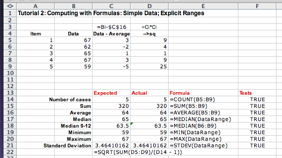
=(Ci=Di) for rows 14 through 21.
Practice these skills and explore the Excel behavior on the following problems: