General Purpose
The term cluster analysis (first used by Tryon, 1939) actually encompasses a number of different classification algorithms. A general question facing researchers in many areas of inquiry is how to organize observed data into meaningful structures, that is, to develop taxonomies. For example, biologists have to organize the different species of animals before a meaningful description of the differences between animals is possible. According to the modern system employed in biology, man belongs to the primates, the mammals, the amniotes, the vertebrates, and the animals. Note how in this classification, the higher the level of aggregation the less similar are the members in the respective class. Man has more in common with all other primates (e.g., apes) than it does with the more "distant" members of the mammals (e.g., dogs), etc. For a review of the general categories of cluster analysis methods, see Joining (Tree Clustering), Two-way Joining (Block Clustering), and K-means Clustering.
Statistical Significance Testing
Note that the above discussions refer to clustering algorithms and do not mention anything about statistical significance testing. In fact, cluster analysis is not as much a typical statistical test as it is a "collection" of different algorithms that "put objects into clusters." The point here is that, unlike many other statistical procedures, cluster analysis methods are mostly used when we do not have any a priori hypotheses, but are still in the exploratory phase of our research. In a sense, cluster analysis finds the "most significant solution possible." Therefore, statistical significance testing is really not appropriate here, even in cases when p-levels are reported (as in k-means clustering).
Area of Application
Clustering techniques have been applied to a wide variety of research problems. Hartigan (1975) provides an excellent summary of the many published studies reporting the results of cluster analyses. For example, in the field of medicine, clustering diseases, cures for diseases, or symptoms of diseases can lead to very useful taxonomies. In the field of psychiatry, the correct diagnosis of clusters of symptoms such as paranoia, schizophrenia, etc. is essential for successful therapy. In archeology, researchers have attempted to establish taxonomies of stone tools, funeral objects, etc. by applying cluster analytic techniques. In general, whenever one needs to classify a "mountain" of information into manageable meaningful piles, cluster analysis is of great utility.
| To index |
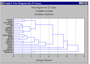
The example in the Introductory Overview illustrates the goal of the joining or tree clustering algorithm. The purpose of this algorithm is to join together objects (e.g., animals) into successively larger clusters, using some measure of similarity or distance. A typical result of this type of clustering is the hierarchical tree.
Hierarchical Tree
Consider a Horizontal Hierarchical Tree Plot (see graph below), on the left of the plot, we begin with each object in a class by itself. Now imagine that, in very small steps, we "relax" our criterion as to what is and is not unique. Put another way, we lower our threshold regarding the decision when to declare two or more objects to be members of the same cluster.
As a result we link more and more objects together and aggregate (amalgamate) larger and larger clusters of increasingly dissimilar elements. Finally, in the last step, all objects are joined together. In these plots, the horizontal axis denotes the linkage distance (in Vertical Icicle Plots, the vertical axis denotes the linkage distance). Thus, for each node in the graph (where a new cluster is formed) we can read off the criterion distance at which the respective elements were linked together into a new single cluster. When the data contain a clear "structure" in terms of clusters of objects that are similar to each other, then this structure will often be reflected in the hierarchical tree as distinct branches. As the result of a successful analysis with the joining method, one is able to detect clusters (branches) and interpret those branches.
Distance Measures
The joining or tree clustering method uses the dissimilarities or distances between objects when forming the clusters. These distances can be based on a single dimension or multiple dimensions. For example, if we were to cluster fast foods, we could take into account the number of calories they contain, their price, subjective ratings of taste, etc. The most straightforward way of computing distances between objects in a multi-dimensional space is to compute Euclidean distances. If we had a two- or three-dimensional space this measure is the actual geometric distance between objects in the space (i.e., as if measured with a ruler). However, the joining algorithm does not "care" whether the distances that are "fed" to it are actual real distances, or some other derived measure of distance that is more meaningful to the researcher; and it is up to the researcher to select the right method for his/her specific application.
Euclidean distance. This is probably the most commonly chosen type of distance. It simply is the geometric distance in the multidimensional space. It is computed as:
distance(x,y) = { i (xi - yi)2 }‡
Note that Euclidean (and squared Euclidean) distances are usually computed from raw data, and not from standardized data. This method has certain advantages (e.g., the distance between any two objects is not affected by the addition of new objects to the analysis, which may be outliers). However, the distances can be greatly affected by differences in scale among the dimensions from which the distances are computed. For example, if one of the dimensions denotes a measured length in centimeters, and you then convert it to millimeters (by multiplying the values by 10), the resulting Euclidean or squared Euclidean distances (computed from multiple dimensions) can be greatly affected, and consequently, the results of cluster analyses may be very different.
Squared Euclidean distance. One may want to square the standard Euclidean distance in order to place progressively greater weight on objects that are further apart. This distance is computed as (see also the note in the previous paragraph):
distance(x,y) = i (xi - yi)2
City-block (Manhattan) distance. This distance is simply the average difference across dimensions. In most cases, this distance measure yields results similar to the simple Euclidean distance. However, note that in this measure, the effect of single large differences (outliers) is dampened (since they are not squared). The city-block distance is computed as:
distance(x,y) = i |xi - yi|
Chebychev distance. This distance measure may be appropriate in cases when one wants to define two objects as "different" if they are different on any one of the dimensions. The Chebychev distance is computed as:
distance(x,y) = Maximum|xi - yi|
Power distance. Sometimes one may want to increase or decrease the progressive weight that is placed on dimensions on which the respective objects are very different. This can be accomplished via the power distance. The power distance is computed as:
distance(x,y) = (i |xi - yi|p)1/r
where r and p are user-defined parameters. A few example calculations may demonstrate how this measure "behaves." Parameter p controls the progressive weight that is placed on differences on individual dimensions, parameter r controls the progressive weight that is placed on larger differences between objects. If r and p are equal to 2, then this distance is equal to the Euclidean distance.
Percent disagreement. This measure is particularly useful if the data for the dimensions included in the analysis are categorical in nature. This distance is computed as:
distance(x,y) = (Number of xi  yi)/ i
Amalgamation or Linkage Rules
At the first step, when each object represents its own cluster, the distances between those objects are defined by the chosen distance measure. However, once several objects have been linked together, how do we determine the distances between those new clusters? In other words, we need a linkage or amalgamation rule to determine when two clusters are sufficiently similar to be linked together. There are various possibilities: for example, we could link two clusters together when any two objects in the two clusters are closer together than the respective linkage distance. Put another way, we use the "nearest neighbors" across clusters to determine the distances between clusters; this method is called single linkage. This rule produces "stringy" types of clusters, that is, clusters "chained together" by only single objects that happen to be close together. Alternatively, we may use the neighbors across clusters that are furthest away from each other; this method is called complete linkage. There are numerous other linkage rules such as these that have been proposed.
Single linkage (nearest neighbor). As described above, in this method the distance between two clusters is determined by the distance of the two closest objects (nearest neighbors) in the different clusters. This rule will, in a sense, string objects together to form clusters, and the resulting clusters tend to represent long "chains."
Complete linkage (furthest neighbor). In this method, the distances between clusters are determined by the greatest distance between any two objects in the different clusters (i.e., by the "furthest neighbors"). This method usually performs quite well in cases when the objects actually form naturally distinct "clumps." If the clusters tend to be somehow elongated or of a "chain" type nature, then this method is inappropriate.
Unweighted pair-group average. In this method, the distance between two clusters is calculated as the average distance between all pairs of objects in the two different clusters. This method is also very efficient when the objects form natural distinct "clumps," however, it performs equally well with elongated, "chain" type clusters. Note that in their book, Sneath and Sokal (1973) introduced the abbreviation UPGMA to refer to this method as unweighted pair-group method using arithmetic averages.
Weighted pair-group average. This method is identical to the unweighted pair-group average method, except that in the computations, the size of the respective clusters (i.e., the number of objects contained in them) is used as a weight. Thus, this method (rather than the previous method) should be used when the cluster sizes are suspected to be greatly uneven. Note that in their book, Sneath and Sokal (1973) introduced the abbreviation WPGMA to refer to this method as weighted pair-group method using arithmetic averages.
Unweighted pair-group centroid. The centroid of a cluster is the average point in the multidimensional space defined by the dimensions. In a sense, it is the center of gravity for the respective cluster. In this method, the distance between two clusters is determined as the difference between centroids. Sneath and Sokal (1973) use the abbreviation UPGMC to refer to this method as unweighted pair-group method using the centroid average.
Weighted pair-group centroid (median). This method is identical to the previous one, except that weighting is introduced into the computations to take into consideration differences in cluster sizes (i.e., the number of objects contained in them). Thus, when there are (or one suspects there to be) considerable differences in cluster sizes, this method is preferable to the previous one. Sneath and Sokal (1973) use the abbreviation WPGMC to refer to this method as weighted pair-group method using the centroid average.
Ward's method. This method is distinct from all other methods because it uses an analysis of variance approach to evaluate the distances between clusters. In short, this method attempts to minimize the Sum of Squares (SS) of any two (hypothetical) clusters that can be formed at each step. Refer to Ward (1963) for details concerning this method. In general, this method is regarded as very efficient, however, it tends to create clusters of small size.
For an overview of the other two methods of clustering, see Two-way Joining and K-means Clustering.
| To index |
Previously, we have discussed this method in terms of "objects" that are to be clustered (see Joining (Tree Clustering)). In all other types of analyses the research question of interest is usually expressed in terms of cases (observations) or variables. It turns out that the clustering of both may yield useful results. For example, imagine a study where a medical researcher has gathered data on different measures of physical fitness (variables) for a sample of heart patients (cases). The researcher may want to cluster cases (patients) to detect clusters of patients with similar syndromes. At the same time, the researcher may want to cluster variables (fitness measures) to detect clusters of measures that appear to tap similar physical abilities.
Two-way Joining
Given the discussion in the paragraph above concerning whether to cluster cases or variables, one may wonder why not cluster both simultaneously? Two-way joining is useful in (the relatively rare) circumstances when one expects that both cases and variables will simultaneously contribute to the uncovering of meaningful patterns of clusters.
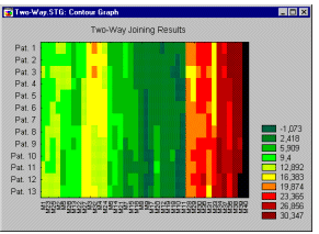
For example, returning to the example above, the medical researcher may want to identify clusters of patients that are similar with regard to particular clusters of similar measures of physical fitness. The difficulty with interpreting these results may arise from the fact that the similarities between different clusters may pertain to (or be caused by) somewhat different subsets of variables. Thus, the resulting structure (clusters) is by nature not homogeneous. This may seem a bit confusing at first, and, indeed, compared to the other clustering methods described (see Joining (Tree Clustering) and K- means Clustering), two-way joining is probably the one least commonly used. However, some researchers believe that this method offers a powerful exploratory data analysis tool (for more information you may want to refer to the detailed description of this method in Hartigan, 1975).
| To index |
This method of clustering is very different from the Joining (Tree Clustering) and Two-way Joining. Suppose that you already have hypotheses concerning the number of clusters in your cases or variables. You may want to "tell" the computer to form exactly 3 clusters that are to be as distinct as possible. This is the type of research question that can be addressed by the k- means clustering algorithm. In general, the k-means method will produce exactly k different clusters of greatest possible distinction.
Example
In the physical fitness example (see Two-way Joining), the medical researcher may have a "hunch" from clinical experience that her heart patients fall basically into three different categories with regard to physical fitness. She might wonder whether this intuition can be quantified, that is, whether a k-means cluster analysis of the physical fitness measures would indeed produce the three clusters of patients as expected. If so, the means on the different measures of physical fitness for each cluster would represent a quantitative way of expressing the researcher's hypothesis or intuition (i.e., patients in cluster 1 are high on measure 1, low on measure 2, etc.).
Computations
Computationally, you may think of this method as analysis of variance (ANOVA) "in reverse." The program will start with k random clusters, and then move objects between those clusters with the goal to (1) minimize variability within clusters and (2) maximize variability between clusters. This is analogous to "ANOVA in reverse" in the sense that the significance test in ANOVA evaluates the between group variability against the within-group variability when computing the significance test for the hypothesis that the means in the groups are different from each other. In k-means clustering, the program tries to move objects (e.g., cases) in and out of groups (clusters) to get the most significant ANOVA results.
Interpretation of results
Usually, as the result of a k-means clustering analysis, we would examine the means for each cluster on each dimension to assess how distinct our k clusters are. Ideally, we would obtain very different means for most, if not all dimensions, used in the analysis. The magnitude of the F values from the analysis of variance performed on each dimension is another indication of how well the respective dimension discriminates between clusters.
| To index |
The methods described here are similar to the k-Means algorithm described above, and you may want to review that section for a general overview of these techniques and their applications. The general purpose of these techniques is to detect clusters in observations (or variables) and to assign those observations to the clusters. A typical example application for this type of analysis is a marketing research study in which a number of consumer behavior related variables are measured for a large sample of respondents. The purpose of the study is to detect "market segments," i.e., groups of respondents that are somehow more similar to each other (to all other members of the same cluster) when compared to respondents that "belong to" other clusters. In addition to identifying such clusters, it is usually equally of interest to determine how the clusters are different, i.e., determine the specific variables or dimensions that vary and how they vary in regard to members in different clusters.
k-means clustering. To reiterate, the classic k-Means algorithm was popularized and refined by Hartigan (1975; see also Hartigan and Wong, 1978). The basic operation of that algorithm is relatively simple: Given a fixed number of (desired or hypothesized) k clusters, assign observations to those clusters so that the means across clusters (for all variables) are as different from each other as possible.
Extensions and generalizations. The EM (expectation maximization) algorithm extends this basic approach to clustering in two important ways:
The EM algorithm for clustering is described in detail in Witten and Frank (2001). The basic approach and logic of this clustering method is as follows. Suppose you measure a single continuous variable in a large sample of observations. Further, suppose that the sample consists of two clusters of observations with different means (and perhaps different standard deviations); within each sample, the distribution of values for the continuous variable follows the normal distribution. The resulting distribution of values (in the population) may look like this:
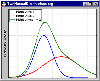
Mixtures of distributions. The illustration shows two normal distributions with different means and different standard deviations, and the sum of the two distributions. Only the mixture (sum) of the two normal distributions (with different means and standard deviations) would be observed. The goal of EM clustering is to estimate the means and standard deviations for each cluster so as to maximize the likelihood of the observed data (distribution). Put another way, the EM algorithm attempts to approximate the observed distributions of values based on mixtures of different distributions in different clusters.
With the implementation of the EM algorithm in some computer programs, you may be able to select (for continuous variables) different distributions such as the normal, log-normal, and Poisson distributions. You can select different distributions for different variables and, thus, derive clusters for mixtures of different types of distributions.
Categorical variables. The EM algorithm can also accommodate categorical variables. The program will at first randomly assign different probabilities (weights, to be precise) to each class or category, for each cluster. In successive iterations, these probabilities are refined (adjusted) to maximize the likelihood of the data given the specified number of clusters.
Classification probabilities instead of classifications. The results of EM clustering are different from those computed by k-means clustering. The latter will assign observations to clusters to maximize the distances between clusters. The EM algorithm does not compute actual assignments of observations to clusters, but classification probabilities. In other words, each observation belongs to each cluster with a certain probability. Of course, as a final result you can usually review an actual assignment of observations to clusters, based on the (largest) classification probability.
| To index |
An important question that needs to be answered before applying the k-means or EM clustering algorithms is how many clusters there are in the data. Remember that the k-means and EM methods will determine cluster solutions for a particular user-defined number of clusters. The k-means and EM clustering techniques (described above) can be optimized and enhanced for typical applications in data mining. The general metaphor of data mining implies the situation in which an analyst searches for useful structures and "nuggets" in the data, usually without any strong a priori expectations of what the analysist might find (in contrast to the hypothesis-testing approach of scientific research). In practice, the analyst usually does not know ahead of time how many clusters there might be in the sample. For that reason, some programs include an implementation of a v-fold cross-validation algorithm for automatically determining the number of clusters in the data.
This unique algorithm is immensely useful in all general "pattern-recognition" tasks - to determine the number of market segments in a marketing research study, the number of distinct spending patterns in studies of consumer behavior, the number of clusters of different medical symptoms, the number of different types (clusters) of documents in text mining, the number of weather patterns in meteorological research, the number of defect patterns on silicon wafers, and so on.
The v-fold cross-validation algorithm applied to clustering. The v-fold cross-validation algorithm is described in some detail in Classification Trees and General Classification and Regression Trees (GC&RT). The general idea of this method is to divide the overall sample into a number of v folds, or randomly drawn (disjointed) sub-samples. The same type of analysis is then successively applied to the observations belonging to the v-1 folds (training sample), and the results of the analyses are applied to sample v (the sample or fold that was not used to estimate the parameters, build the tree, determine the clusters, etc.; this is the testing sample) to compute some index of predictive validity. The results for the v replications are aggregated (averaged) to yield a single measure of the stability of the respective model, i.e., the validity of the model for predicting new observations.
Cluster analysis is an unsupervised learning technique, and we cannot observe the (real) number of clusters in the data. However, it is reasonable to replace the usual notion (applicable to supervised learning) of "accuracy" with that of "distance." In general, we can apply the v-fold cross-validation method to a range of numbers of clusters in k-means or EM clustering, and observe the resulting average distance of the observations (in the cross-validation or testing samples) from their cluster centers (for k-means clustering); for EM clustering, an appropriate equivalent measure would be the average negative (log-) likelihood computed for the observations in the testing samples.
Reviewing the results of v-fold cross-validation. The results of v-fold cross-validation are best reviewed in a simple line graph.
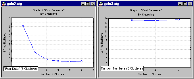
Shown here is the result of analyzing a data set widely known to contain three clusters of observations (specifically, the well-known Iris data file reported by Fisher, 1936, and widely referenced in the literature on discriminant function analysis). Also shown (in the graph to the right) are the results for analyzing simple normal random numbers. The "real" data (shown to the left) exhibit the characteristic scree-plot pattern (see also Factor Analysis), where the cost function (in this case, 2 times the log-likelihood of the cross-validation data, given the estimated parameters) quickly decreases as the number of clusters increases, but then (past 3 clusters) levels off, and even increases as the data are overfitted. Alternatively, the random numbers show no such pattern, in fact, there is basically no decrease in the cost function at all, and it quickly begins to increase as the number of clusters increases and overfitting occurs.
It is easy to see from this simple illustration how useful the v-fold cross-validation technique, applied to k-means and EM clustering can be for determining the "right" number of clusters in the data.
| To index |