Problems
Given a query Q and a collection of documents A, B and C shown in Table 1, find the similarity among each one of the documents and the query (i.e. sim(A,Q), sim(B,Q) and sim(C,Q)) by using the cosine similarity metric and then rank the three documents based on these similarity values.
The numbers in the table are the TF-IDF weights of each term in each document and in the query; simply compute the cosine similarity using these TF-IDF weights.
Table 1. TF-IDF Weights
|
Cat |
Food |
Fancy |
Q |
3 |
4 |
1 |
A |
2 |
1 |
0 |
B |
1 |
3 |
1 |
C |
0 |
2 |
2 |
Given a query Q and a collection of documents A, B, and C as shown in Table 2, determine the similarity between the documents and the query using language modeling. In particular compute the (log of the) probability of generating the query Q from the language model defined by each document, using the simple unigram language, the multinomial model (i.e. the probability of a query being generated is equal to the product of the probabilities of generating each term in the query) and the following smoothing techniques:
- No smoothing, i.e. maximum likelihood language model.
- Laplace smoothing.
- Witten-Bell smoothing. For the corpus model, use the average of the maximum likelihood models created in part (a).
The numbers in the table below are now the raw term frequencies in each document and in the query. Note that if a term appears more than once in the query, it will have to be "generated" more than once in the simple multinomial model.
Table 2. Term Frequencies
|
Cat |
Food |
Fancy |
Q |
3 |
4 |
1 |
A |
2 |
1 |
0 |
B |
1 |
3 |
1 |
C |
0 |
2 |
2 |
-
In this homework problem, you will write a quick program to explore
Zipf's Law.
Go to the Project Gutenberg website and download Alice in Wonderland by Lewis Carol. Strip off the header, and thus consider only the text starting at "ALICE'S ADVENTURES IN WONDERLAND", just preceding "CHAPTER 1"; also, strip off the footer, eliminating the license agreement and other extraneous text, and thus consider only the text up through, and including, "THE END". Use this perl script to strip the text of punctuation obtaining the original text as a list of words. For example, on a unix based systems, you should run a command like
parse.pl alice30.txt > output
Write a quick program or script that counts word frequencies. For the most frequent 25 words and for the most frequent 25 additional (i.e. not in the first set) words that start with the letter f (a total of 50 words), print the word, the number of times it occurs, its rank in the overall list of words, the probability of occurrence, and the product of the rank and the probability. Also indicate the total number of words and the total number of unique words that you found. Discuss whether this text satisfies Zipf's Law. Feel free to use other parts of the ranked list of terms.
- Suppose that while you were building a retrieval index, you decided to omit all the words that occur less than five times (i.e., one to four times). According to Zipf's Law, what proportion of the total (i.e. not total unique) words in the collection would you omit? (Justify your answer.) What proportion would actually be omitted in the Alice in Wonderland text above?
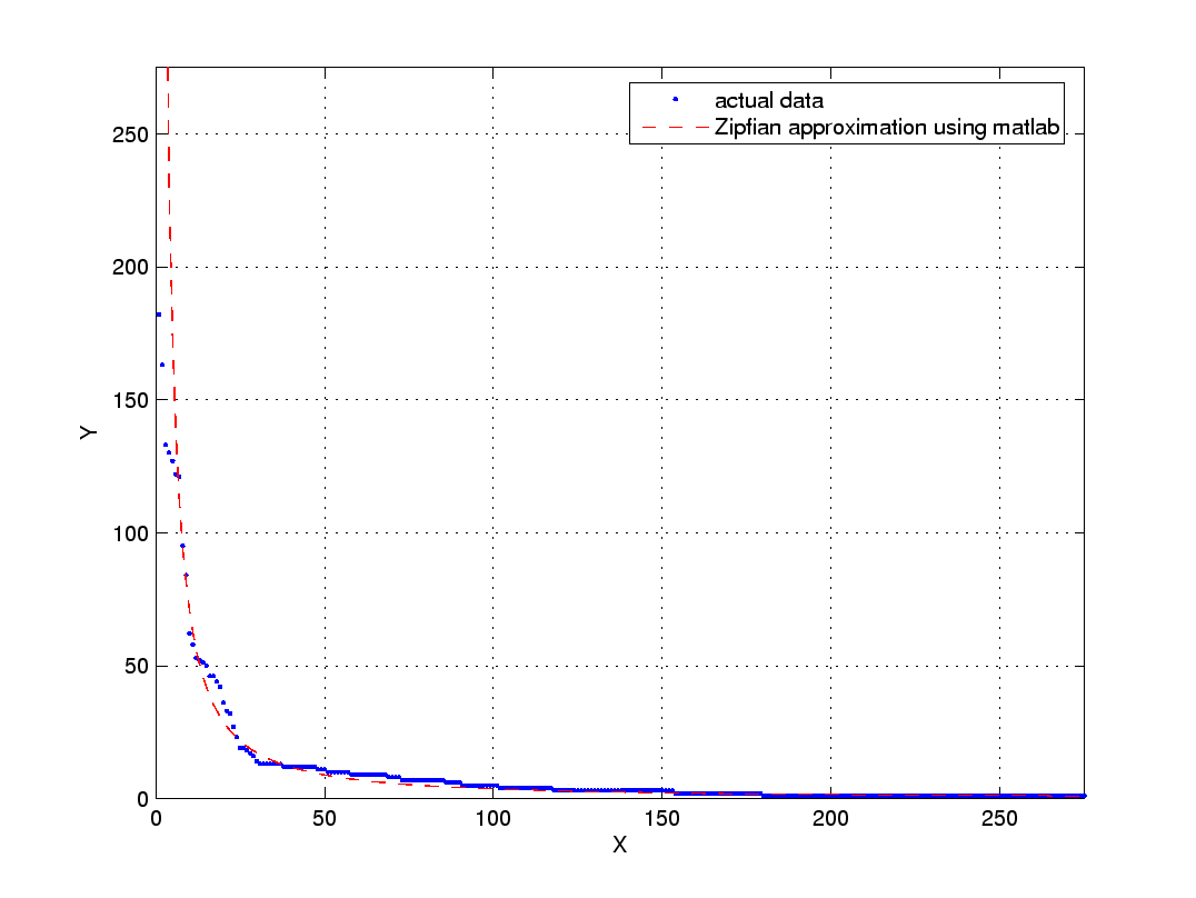
Prof. Aslam has a collection of songs on his iPod, each song played a number of times as indicated in this ranked list
The left plot below show the frequence-rank plot for these songs (the blue dots) along with a "best fit" Zipfian model (red curve). The right plot shows this same data on a log-log scale.
 |
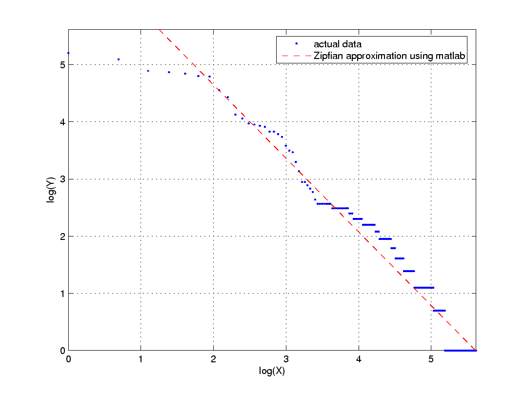 |
| Figure 1(a). Frequency-rank plot and best fit Zipfian model. | Figure 1(b). Log-log plot of data from Figure 1(a). |
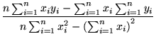
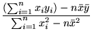
Your task is to find the best fit Zipfian model for this data, i.e., the parameters of the red curve, by first finding the best fitting straight line for the log-log data using the least squares technique. Follow the detailed example given in class. As a reminder, if the log-log data points are represented by
and you are looking for the linear function (straight line) given by
then
 |
 |
|||
 |
 |
- According to Heaps' Law, what proportion of a collection of text must be read before 90% of its vocabulary has been encountered? You may assume that beta=0.5. Hint: to solve this problem you don't need to know the value of K.
- Verify Heap's Law on the Alice in Wonderland text. Process each word of the text, in order, and compute the following pairs of numbers: (number of words processed, number of unique words seen). These pairs of numbers, treated as (x,y) values, should satisfy Heaps Law. Appropriately transform the data and use least squares to determine the model parameters K and beta, in much the same manner as Zipf's Law example from class and the problem above.