- Examine the characteristics of five different real world graphs
- These graphs all come from different domains
- Most were not designed to have specific properties
- All grew organically
- You would not expect them to have structure or be similar to each other
- Evaluation metrics
- Degree distribution, assortativity
- Clustering coefficient
- Shortest paths distances, eccentricity
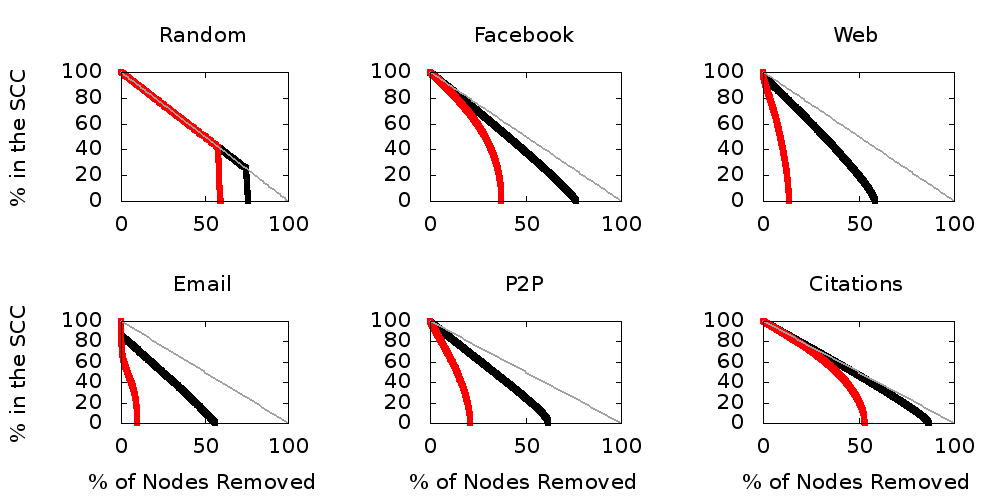
- Resiliency against node removal
- Compare against a synthetic baseline
Real World Graphs
How do we analyze graphs?
How do different graphs compare?
What makes graphs "special"?
Goals
Cast of Characters
- Facebook: Snapshot of Mexico regional network
- Nodes: 598140, Edges: 4552493, Collected: 2009
- Web: Web graph subsample from Google
- Nodes: 875713, Edges: 5105039, Collected: 2002
- Email: Complete email communication network from Enron
- Nodes: 36692, Edges: 183831, Collected: 2004
- P2P: Complete Gnutella peer to peer network
- Nodes: 62586, Edges: 147892, Collected: August 31 2002
- Citations: Complete Arxiv high energy physics citation graph
- Nodes: 34546, Edges: 421578, Collected: 2003
Choosing a Baseline for Comparison
Which graph type best corresponds with real world graphs?
Complete graph
Ring
Star
Tree
Bipartite
Random
Random Graphs
- Graphs we will study are considered to be random graphs
- Very sparse (i.e. not complete)
- Not "designed" to have structure (i.e. not a ring or star)
- Not heirarchical (i.e. not a tree)
- Not divided into classes of nodes (i.e. not bipartite)
- Random graph generation
- Known as an Erdős-Rényi graphs, or binomial graphs
- \(G_{n, p}\): Choose number of nodes \(n\) and probability \(p\)
- Form each edge \((u, v) \in G\) with probability \(p\)
- Graph used in these experiments
- \(G_{10000, 0.001}\) -- Nodes: 10000, Edges: 100000
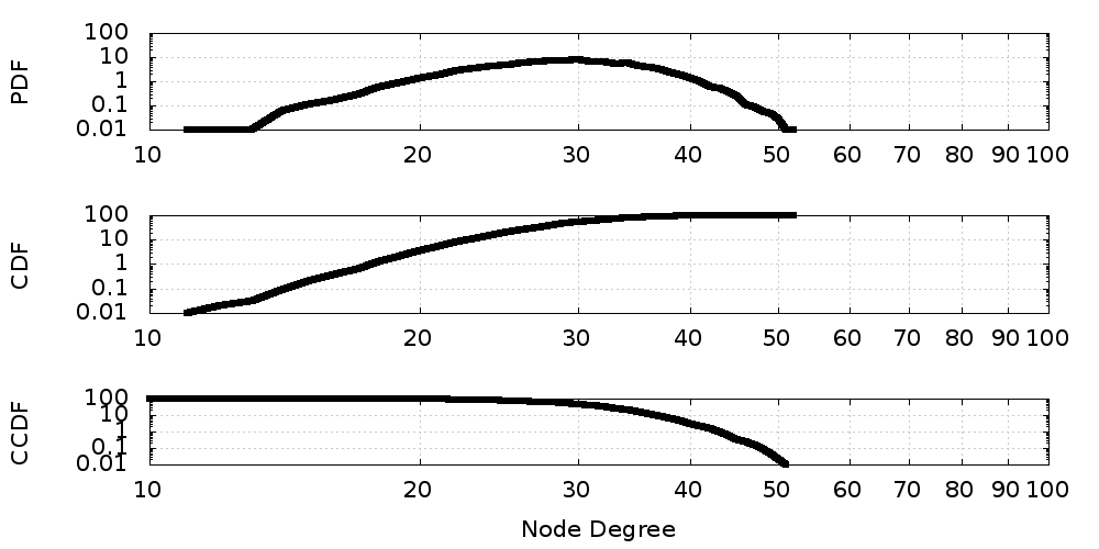
How to read PDFs, CDFs, and CCDFs
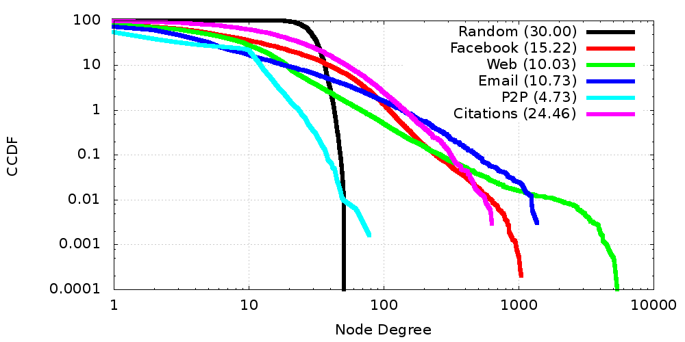
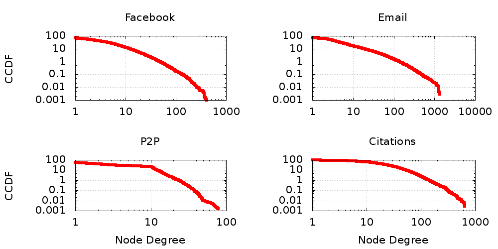
Degree Distributions (CCDF)
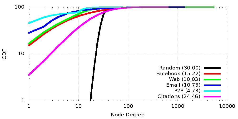
Degree Distributions (CDF)
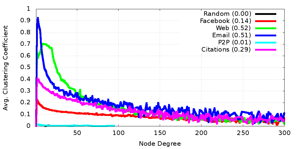
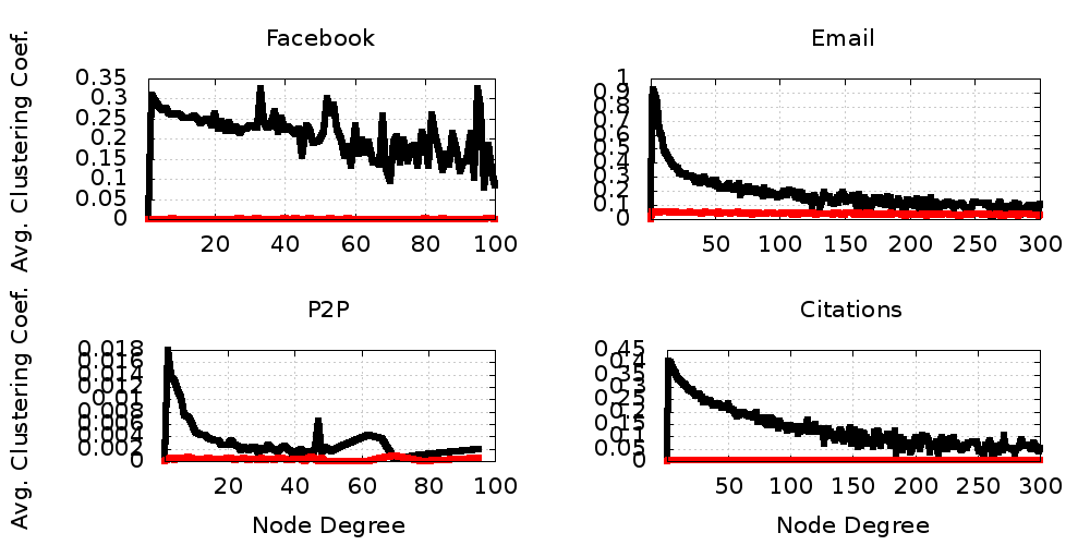
Clustering Coefficient
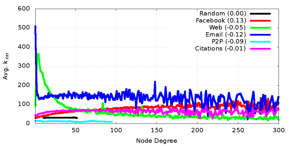
\(k_{nn}\) and Assortativity
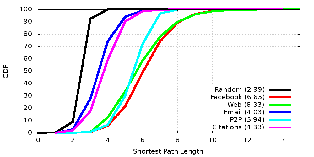
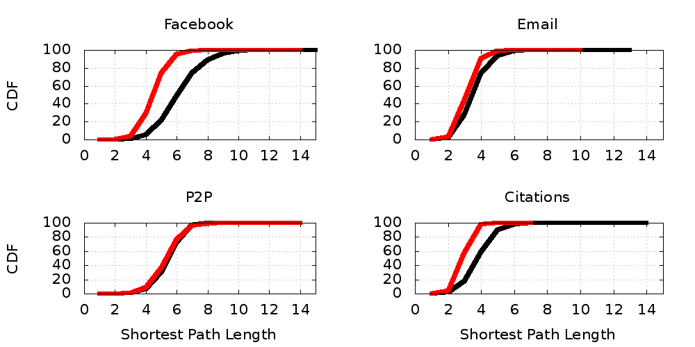
Shortest Path Distances
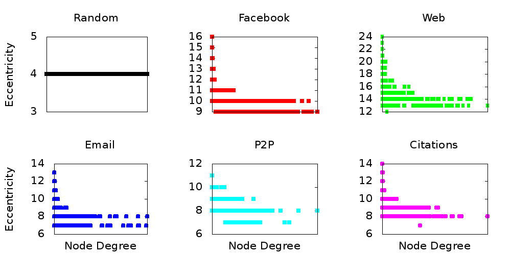
Eccentricity
Resiliency
Takeaways So Far...
- Real world graphs are significantly different from random graphs
- Degree distributions have long tails
- Many, many low degree nodes...
- But also a small core of high-degree super-nodes
- Small-world phenomenon
- More clustering than a random graph...
- But also relatively short average path lengths
- Known as the tightly-clustered fringe
- Degree distributions have long tails
- Significant variations of characteristics among real world graphs
- No single metric tells the whole story about a graph
What is so important about the degree distribution?
- Great deal of focus in the literature on the degree distribution
- Especially power-law degree distributions
- Are other metrics "linked" to the degree distribution?
- Conduct an experiment
- Take real graphs and re-wire them
- Each node maintains its original degree...
- But the endpoints of all the edges change
Degree Distributions
Shortest Path Distances
Clustering Coefficient
Takeaways
- Long tailed degree distributions are prevelent in real world graphs
- We would not expect real world graphs to have this feature
- That so many graphs do tells us this is an important, emergent characteristic
- But degree distribution is not the whole story
- Clustering, path lengths, assortativity, etc. are equally important
- These metrics are not dependent on the degree distribution
Modeling Real World Graphs
Understanding Emergent Graph Properties
- Real world graphs have many unexpected features
- Long tailed degree distributions
- Tightly clustered fringes
- Short average path lengths
- Resiliency against random destruction
- What natural process creates graphs with these characteristics?
- Understanding this process can lead to great insight about the natural world
- Applicable to many domains, e.g. biology, sociology, computer science, etc.
Graph Models
- Key idea:
- Create a simple model that generates graphs with desired characteristics
- Intuition behind algorithm (hopefully) reflects real world processes
- Example from physics: \(F = m * a\)
- Extremely simple model, only three variables
- Enables us to predict projectile motion, celestial orbits, etc.
- Imparts fundamental understanding about the laws and relationships in nature
Erdős-Rényi Model
- Introduced in 1959
- Generate a uniformly random graph
- \(G_{n, p} = (V, E)\)
- \(n = |V|\)
- Form each edge \((u, v) \in E\) with probability \(p\)
- Not a good fit for real world graphs
- Short-tailed degree distribution
- Zero clustering
- Assortativity is zero
- Path lengths are too short
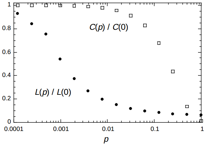
Watts-Strogatz Model
- Introduced in 1998
- Key ideas
- Start with a uniform, tightly clustered graph (a ring lattice)
- Randomly rewire edges to introduce "shortcuts"
- Resulting graph is still highly clustered, but also has short path lengths
- Model parameters
- \(G_{n, k, p} = (V, E)\)
- \(n = |V|\)
- Connect each node to its \(k\) nearest neighbors in the ring
- Rewire each edge \((u, v) \in E\) to \((u, v')\) where \(v' \in V\) with probability \(p\)
- Resulting graphs is small-world
- But does not have a power-law degree distribution
Example Watts-Strogatz Graph
Parameters: \(G_{30, 4, 0}\)
Avg. Path Len: 4.14
Avg. Clustering: 0.5
Average Path Length vs. Clustering Coefficient
Barabási-Albert Model
- Introduced in 1999
- Sometimes called Preferential Attachment
- Exhibits a rich-get-richer pattern
- Model parameters
- \(G_{n, m} = (V, E)\)
- \(n = |V|\)
- Connect each node to \(m\) other nodes
- Probability of connecting to node \(i\) with degree \(k_i\): \(\Pi(k_i) = \frac{k_i}{\sum\limits_{j \in V} k_j}\)
- Resulting graphs has:
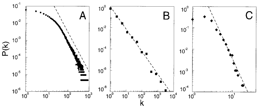
- Power-law degree distribution \(P(k) \sim k^{-\gamma}\)
- Scale-free behavior
Power-laws In Action
Nearest Neighbor Model
- Introduced in 2003
- Based on intuition about social dynamics
- Your friends are likely to be friends with each other
- Model parameters
- \(G_{n, u} = (V, E)\)
- \(n = |V|\)
- With probability \(u\), add a new node and connect it to a random node
- Otherwise, randomly close a triangle in the graph
- Resulting graphs has:
- Power-law degree distribution with \(\gamma > 2\)
- Tighly-clustered fringe
Many, Many Graph Models
- Random Walk Model (2003)
- Emulates pattern of friend discovery in social networks
- Add a new node \(v\), and begin a random walk starting at a random node
- At each step of the walk, connect \(v\) to that node with probability \(q_v\)
- Forest Fire Model (2005)
- Builds graphs with diameters that shrink as they grow larger
- Add a new node \(v\), and randomly connect it to a node \(w\)
- With probability \(p\), "burn" (i.e. connect) \(v\) to each of \(w\)'s neighbors
- Continue this process recursively from each burned node
Fitting Models to Real World Graphs
- d\(k\) Model (2006)
- Precisely captures real world graphs using joint degree distributions
- d\(k\)-1: degree distribution
- d\(k\)-2: joint degree distribution
- d\(k\)-3: tri-degree distribution (captures clustering)
- etc.
- Very accurate, but very costly
- State-space (i.e. memory) explodes as \(k\) increases
- Graph generators for \(k \ge 3\) do not currently exist
- Precisely captures real world graphs using joint degree distributions
- Kronecker Graphs (2007)
- Uses Kronecker multiplication to recursively "evolve" an initiator graph
- Use MLE to fit the evolved graph to a real world graphs
Microscopic Model
- Introduced in 2008
- Models dynamic graphs that grow over time
- Model parameters: \(N()\), \(\lambda\), \(\alpha\), \(\beta\)
- Node arrival function \(N()\), typically a quadratic over time \(t\)
- On arrival, node \(v\) samples its lifetime \(a_v = \lambda \mathrm{e}^{-\lambda}\)
- Attach \(v\) using preferential attachment
- Node \(v\) with degree \(d_v\) samples it sleep-time from \(p_v = d_v^{-\alpha} * \beta d_v \mathrm{e}^{-\beta d_v}\)
- When \(v\) wakes up, if its lifetime has not expired, close a triangle that includes \(v\)
- Complicated model, but produces power-law, tightly clustered graphs
- One of very few models that models dynamic graphs over time
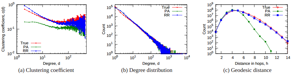
Microscopic Model In Action
Comparing Preferential Attachment (PA) and Microscopic Model (RR) to the actual Flickr social graph
Discussion
- Which model produces the most realistic graphs?
- That depends on what kind of graph you want
- Different models produce graphs that emphasize different metrics
- Power-law degree distribution
- Clustered fringe
- Shrinking diameter
- etc.
- How do you get the best, most realistic graphs from models?
- Most models have lots of parameters. How do you choose the right values?
- Some models are designed to fit real graphs, but these models are very expensive